James Barabas for MAS622J Fall 2004
For my project, I examined a set of data taken from eye movement recordings performed at the Schepens Eye Research Institute. The recordings were made in an effort to understand the differences between subjects' viewing patterns as they watched television. In the original experiment, data were recorded from 26 subjects in 30 minute sessions. In each session, subjects watched on a television a sequence of six five-minute video sequences taken from Hollywood movies. Eye movements were recorded using a video eye tracking system. Raw eye movement data consisted of measurements of two-dimensional eye position on the video screen (511 units in each dimension), and measurements were taken 60 times per second.
I used this data to examine the differences in the distributions of eye position between the different video sequences. Specifically, I examined different methods for identifying video sequences from eye movement data.
For most methods, I divided the subjects into a 22 subject training group and a 4 subject validation group. Since each subject watched six different video sequences, there were 132 training sequences and 24 test sequences. I used my own Matlab code and paramater optimization routines from the Optimization Toolbox to perform my experiments.
Since eye movements are recorded continuously over time, eye movement classification might lend itself well to analysis by Hidden Markov Models. I experimented with a few simple HMMs. Each HMM contained a linear sequence of states where transitions were only possible from a given state to its neighbor to the right. Subjects were assumed to start in the leftmost state at the start of the video sequences. I tested models with up to 15 states using data from the first 100 samples of the six video sequences. Data from the set of 22 training subjects were used to train the HMMs.
To build a set of symbols, I binned eye movement data. I divided the video frame into a 5x5 grid, and considered eye position measurements falling on each grid square to represent a different symbol. In this way, eye movement recordings from each session were reduced to a time series of symbols drawn from an alphabet of 25.
Classification results for test subjects (2-D bins):
Subject 23
| Sequence: | 1 | 2 | 3 | 4 | 5 | 6 |
|---|
| 1 state HMM: | 1 | 2 | 3 | 4 | 5 | 6 |
| 2 state HMM: | 1 | 2 | 2 | 4 | 5 | 6 |
| 3 state HMM: | 1 | 2 | 6 | 4 | 5 | 6 |
| 4 state HMM: | 1 | 2 | 2 | 4 | 5 | 6 |
| 5 state HMM: | 1 | 2 | 6 | 4 | 5 | 6 |
Subject 24
| Sequence: | 1 | 2 | 3 | 4 | 5 | 6 |
|---|
| 1 state HMM: | 1 | 2 | 3 | 4 | 5 | 6 |
| 2 state HMM: | 1 | 2 | 3 | 4 | 5 | 6 |
| 3 state HMM: | 1 | 2 | 3 | 4 | 5 | 6 |
| 4 state HMM: | 1 | 2 | 1 | 4 | 5 | 6 |
| 5 state HMM: | 1 | 2 | 1 | 4 | 5 | 6 |
Subject 25
| Sequence: | 1 | 2 | 3 | 4 | 5 | 6 |
|---|
| 1 state HMM: | 1 | 6 | 3 | 4 | 5 | 6 |
| 2 state HMM: | 6 | 6 | 3 | 4 | 5 | 6 |
| 3 state HMM: | 1 | 2 | 3 | 4 | 5 | 6 |
| 4 state HMM: | 1 | 1 | 3 | 4 | 5 | 6 |
| 5 state HMM: | 1 | 1 | 3 | 4 | 5 | 6 |
Subject 26
| Sequence: | 1 | 2 | 3 | 4 | 5 | 6 |
|---|
| 1 state HMM: | 1 | 2 | 3 | 4 | 5 | 6 |
| 2 state HMM: | 1 | 2 | 3 | 4 | 5 | 6 |
| 3 state HMM: | 1 | 2 | 3 | 4 | 5 | 6 |
| 4 state HMM: | 1 | 2 | 3 | 4 | 5 | 6 |
| 5 state HMM: | 1 | 2 | 3 | 4 | 5 | 6 |
I also tried using a set of symbols that encoded time information as well. I binned the data into a volume of 5x5 bins in screen space, by 10 bins in time. This way, eye fixations made to the same part of the screen at a later time would represent two different symbols. Although training took longer, results were good even with three-state models. This makes sense, as the matrix of symbol probabilities in a simple HMM state model are much like an estimate of the 3-D density function in position and time.
Classification results for test subjects (3-D bins):
Subject 23
| Sequence: | 1 | 2 | 3 | 4 | 5 | 6 |
|---|
| 1 state HMM: | 1 | 2 | 3 | 4 | 5 | 6 |
| 2 state HMM: | 1 | 2 | 2 | 4 | 5 | 6 |
| 3 state HMM: | 1 | 2 | 6 | 4 | 5 | 6 |
| 4 state HMM: | 1 | 2 | 2 | 4 | 5 | 6 |
| 5 state HMM: | 1 | 2 | 6 | 4 | 5 | 6 |
| 10 state HMM: | 1 | 2 | 6 | 4 | 5 | 6 |
| 15 state HMM: | 1 | 2 | 6 | 4 | 5 | 6 |
Subject 24
| Sequence: | 1 | 2 | 3 | 4 | 5 | 6 |
|---|
| 1 state HMM: | 1 | 2 | 3 | 4 | 5 | 6 |
| 2 state HMM: | 1 | 2 | 3 | 4 | 5 | 6 |
| 3 state HMM: | 1 | 2 | 3 | 4 | 5 | 6 |
| 4 state HMM: | 1 | 2 | 1 | 4 | 5 | 6 |
| 5 state HMM: | 1 | 2 | 1 | 4 | 5 | 6 |
| 10 state HMM: | 1 | 2 | 1 | 4 | 5 | 6 |
| 15 state HMM: | 1 | 2 | 1 | 4 | 5 | 6 |
Subject 25
| Sequence: | 1 | 2 | 3 | 4 | 5 | 6 |
|---|
| 1 state HMM: | 1 | 6 | 3 | 4 | 5 | 6 |
| 2 state HMM: | 6 | 6 | 3 | 4 | 5 | 6 |
| 3 state HMM: | 1 | 2 | 3 | 4 | 5 | 6 |
| 4 state HMM: | 1 | 1 | 3 | 4 | 5 | 6 |
| 5 state HMM: | 1 | 1 | 3 | 4 | 5 | 6 |
| 10 state HMM: | 1 | 1 | 3 | 4 | 5 | 6 |
| 15 state HMM: | 1 | 2 | 3 | 4 | 5 | 6 |
Subject 26
| Sequence: | 1 | 2 | 3 | 4 | 5 | 6 |
|---|
| 1 state HMM: | 1 | 2 | 3 | 4 | 5 | 6 |
| 2 state HMM: | 1 | 2 | 3 | 4 | 5 | 6 |
| 3 state HMM: | 1 | 2 | 3 | 4 | 5 | 6 |
| 4 state HMM: | 1 | 2 | 3 | 4 | 5 | 6 |
| 5 state HMM: | 1 | 2 | 3 | 4 | 5 | 6 |
| 10 state HMM: | 1 | 2 | 3 | 4 | 5 | 6 |
| 15 state HMM: | 1 | 2 | 3 | 4 | 5 | 6 |
Next, I tried using Parzen Windows to estimate the density function of eye position in the video frame. First, I discarded all time information and only considered the 2-D position of eye fixations. I used a 2-D uncorrelated Gaussian distributions as the window function, and estimated the 2-D probability density function of eye position in the video frame. I used 3600 samples (the first minute of video) from each video sequence watched by the 22 training subjects to build the density estimates.
| Sequence: | 1 | 2 | 3 | 4 | 5 | 6 |
|---|
| Subject 23: | 1 | 2 | 1 | 4 | 5 | 2 |
| Subject 24: | 1 | 2 | 3 | 4 | 5 | 6 |
| Subject 25: | 1 | 2 | 6 | 4 | 6 | 6 |
| Subject 26: | 1 | 4 | 3 | 4 | 6 | 6 |
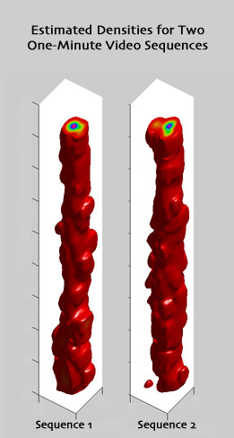
I was curious to see what the 3-D density functions (eye position in two dimensions on screen as well as in time) so I also performed some experiments with 3-D Parzen windows. Here, I used tri-variate Gaussian distributions with diagonal covariance matrices. Since space and time are measured in different units, I decided to solve for the parameters of a covariance matrix to model the relative variation in the three measured dimensions.
To find the 3-D Parzen window parameters, I took a set of ten subjects (from only one of the six video sequences, ideally, this would have been done using the entire training set, and all video sequences). Using leave-one-out validation and Levenberg Marquardt optimization, I found the set of parameters that maximized the sum of likelihoods over all ten test datasets when trained using the remaining nine. (This took a long time.) In future experiments, it would be interesting to see the result of alternatively maximizing classification performance within the same 10-subject group.
Classification Results for max likelihood in 3D:
| Sequence: | 1 | 2 | 3 | 4 | 5 | 6 |
|---|
| Subject 23: | 1 | 4 | 1 | 4 | 5 | 2 |
| Subject 24: | 1 | 2 | 1 | 4 | 6 | 6 |
| Subject 25: | 1 | 1 | 3 | 2 | 5 | 5 |
| Subject 26: | 1 | 2 | 3 | 4 | 2 | 6 |
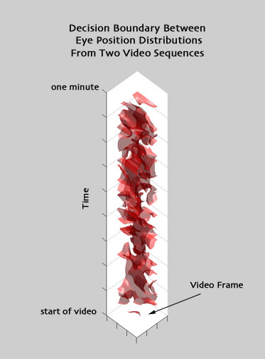
After solving for the window parameters, I was able to compute some visualizations of the shape of the 3-D density function. Plotted in red are surfaces of equal density in screen-position and time, with slices showing relative probability density at the boundaries of the plotted domain: