
Does the way that people speak at the same time (or almost the same time) yield information about which speakers have opposing or supporting viewpoints?
2 classes : agreed, opposed
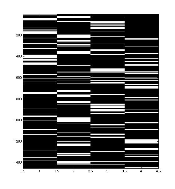
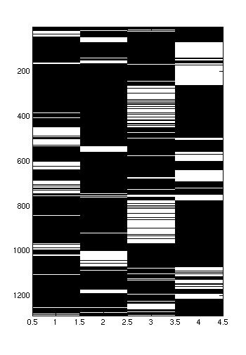
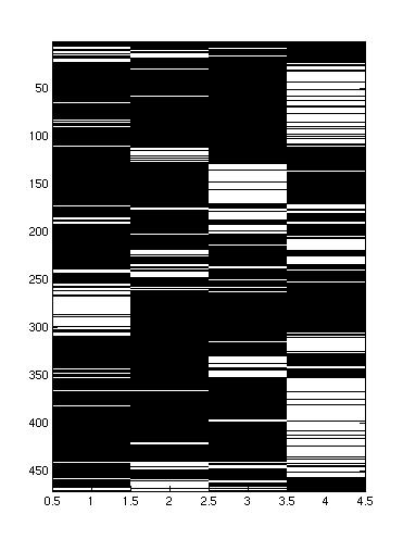
Transformed original data into 4 vectors.
+1 if person spoke
-1 if person did not speak
Correlation of 4 by T matrix
Each element of the correlation matrix indicates how frequently two people spoke at the same time.
In a given conversation, if the labels for two individuals are the same, take the correlation of the times when they spoke, and add that to the "agreed" class.
If the labels are not the same, take the correlation of the times when they spoke, and add that to the "opposed" class.
69 points of training data
74 points of testing data
* Allies will tend to speak at the same time, supporting eachother's point, and making noises to indicate agreement.
* Opponents will not speak at the same time, taking clear turns, exchanging information and ideas.
* There will be roughly two clusters of correlations, one for allies, and one for opponents. The correlations between allies will be higher than the correlations between opponents.
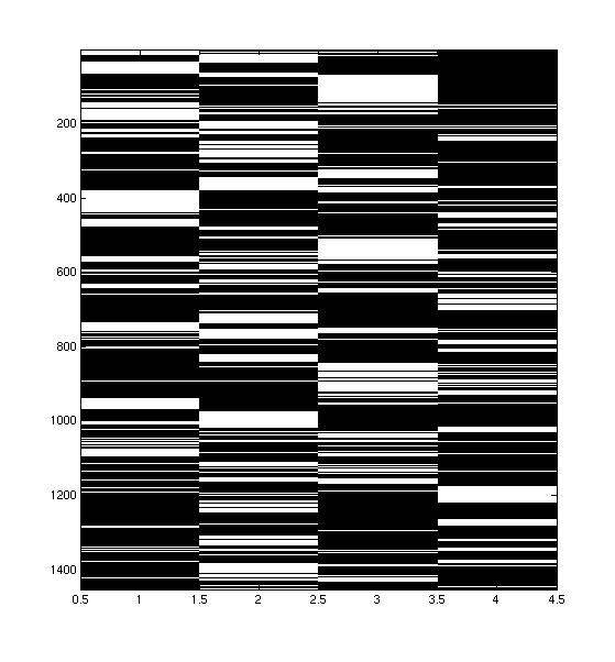
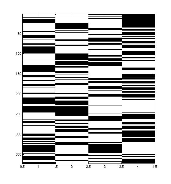
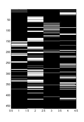
I believed that the times when people spoke at the same time were important, and so I decided that I wanted to exaggerate the times when people spoke at the same time. I used three methods to do this:
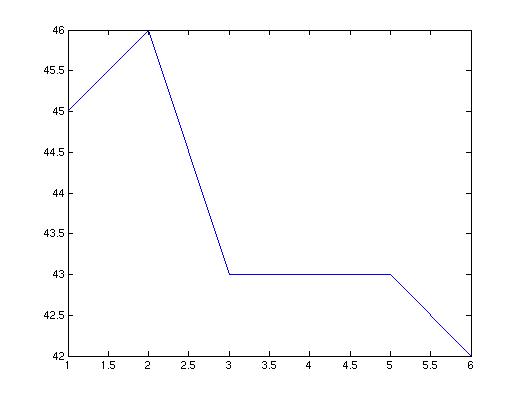
| Original Conversation | Smoothed Conversation |
| |
|
| Compressed Conversation | Conversation Interference |
|
|
My first task was to try to improve the discriminability of the classes. This was done by choosing a set of parameters to use with each classification method, and then selecting the mode of pre-processing that led to the most consistently high performance across classifiers. I found that the pre-processing that led to the best discriminability was compression of the conversations, after they were smoothed with a sliding window of width 10.
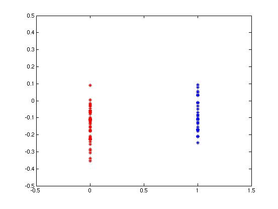
Below, the classes derived from the original, unprocessed data are shown. The table below shows how each classifier performed on data that had been subjected to different styles of pre-processing. The selected mode is highlighted.
 |
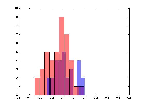 |
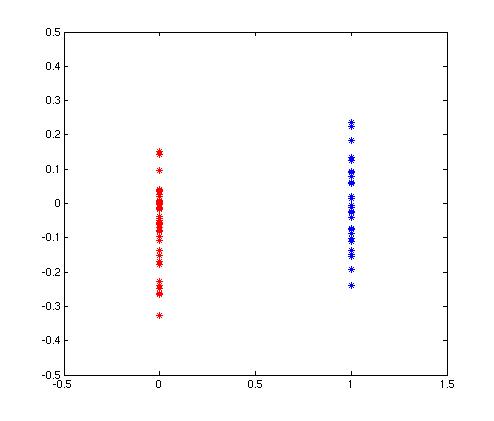
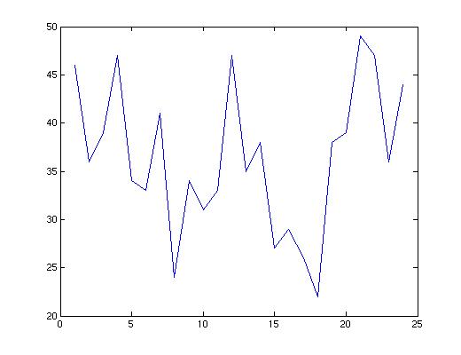
| Plot and histogram of correlations from raw, un-processed data | |
| class1: correct, incorrect class2: correct, incorrect all: correct, incorrect |
Parzen, h = 0.25 | Parzen, h = 0.125 | Parzen, h = 0.0625 | KNN, k = 2 | KNN, k = 4 | KNN, k = 20 | GLD, k = 3 | GLD, k = 4 | GLD, k = 5 |
| Raw Data | 18, 10 21, 20 39, 30 |
18, 10 21, 20 39, 30 |
20, 8 18, 23 38, 31 |
14, 14 24, 17 38, 31 |
25, 3 1, 40 26, 43 |
2, 26 37, 4 39, 30 |
6, 22 39, 2 45, 24 |
6, 22 39, 2 45, 24 |
8, 20 39, 2 47, 22 |
| Sliding window, width = 3 |
18, 10 17, 24 35, 34 |
23, 5 14, 27 37, 32 |
22, 6 15, 26 37, 32 |
23, 5 7, 34 30, 39 |
23, 5 5, 36 28, 41 |
0, 28 39, 2 39, 30 |
3, 25 40, 1 43, 26 |
2, 26 40, 1 42, 27 |
3, 25 40, 1 43, 26 |
| Sliding window, width = 5 |
19, 9 16, 25 35, 34 |
24, 4 10, 31 34, 35 |
23, 5 20, 21 43, 26 |
23, 5 6, 35 29, 40 |
21, 7 8, 33 29, 40 |
2, 26 40, 1 42, 27 |
2, 26 40, 1 42, 27 |
2, 26 40, 1 42, 27 |
2, 26 40, 1 42, 27 |
| Sliding window, width = 10 |
19, 9 12, 29 31, 38 |
25, 3 21, 20 46, 23 |
23, 5 23, 18 46, 23 |
23, 5 6, 35 29, 40 |
25, 3 4, 37 29, 40 |
1, 27 40, 1 41, 28 |
2, 26 39, 2 41, 28 |
3, 25 39, 2 42, 27 |
6, 22 38, 3 44, 25 |
| Compressed after Sliding window, width = 3 |
14, 14 23, 18 37, 32 |
23, 5 16, 25 39, 30 |
26, 2 15, 26 41, 28 |
26, 2 4, 37 30, 39 |
19, 9 11, 30 30, 39 |
13, 15 29, 12 42, 27 |
6, 22 37, 4 43, 26 |
5, 23 38, 3 43, 26 |
4, 24 41, 0 45, 24 |
| Compressed after Sliding window, width = 5 |
11, 17 31, 10 42, 27 |
15, 13 25, 16 40, 29 |
23, 5 15, 26 38, 31 |
27, 1 1, 40 28, 41 |
25, 3 1, 40 26, 43 |
2, 26 41, 0 43, 26 |
8, 20 37, 4 45, 24 |
8, 20 39, 2 47, 22 |
8, 20 39, 2 47, 22 |
| Compressed after Sliding window, width = 10 |
13, 15 28, 13 41, 28 |
11, 17 33, 8 44, 25 |
10, 18 36, 5 46, 23 |
27, 1 0, 41 27, 42 |
8, 20 35, 6 43, 26 |
7, 21 40, 1 47, 22 |
5, 23 39, 2 44, 25 |
7, 21 38, 3 45, 24 |
7, 21 38, 3 45, 24 |
| Interference after Sliding window, width = 3 |
25, 3 12, 29 37, 32 |
25, 3 12, 29 37, 32 |
24, 4 14, 27 38, 31 |
25, 3 5, 36 30, 39 |
8, 20 30, 11 38, 31 |
23, 5 16, 25 39, 30 |
0, 28 41, 0 41, 28 |
1, 27 41, 0 42, 27 |
1, 27 41, 0 42, 27 |
| Interference after Sliding window, width = 5 |
20, 8 19, 22 39, 30 |
21, 7 17, 24 38, 31 |
20, 8 19, 22 39, 30 |
22, 6 8, 33 30, 39 |
3, 25 37, 4 40, 29 |
16, 12 21, 20 37, 32 |
1, 27 40, 1 41, 28 |
1, 27 40, 1 41, 28 |
1, 27 40, 1 41, 28 |
| Interference after Sliding window, width = 10 |
8, 20 32, 9 40, 29 |
15, 13 24, 17 39, 30 |
20, 8 18, 23 38, 31 |
26, 2 4, 37 30, 39 |
8, 20 32, 9 40, 29 |
6, 22 37, 4 43, 26 |
5, 23 37, 4 42, 27 |
5, 23 38, 3 43, 26 |
2, 26 39, 2 41, 28 |
 |
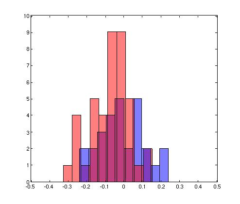 |
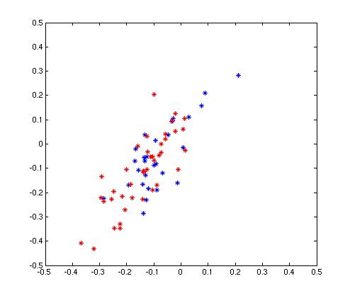
| A scatter plot and histogram of the points in each of the two classes of data. Points for individuals that agreed with each other are shown in blue. Points for individuals that disagreed with each other are shown in red. | |
Once I fixed the mode of pre-processing, I tried to identify which style of classifier would suit my data best. I chose between Parzen windows, K-nearest neighbors, and general linear discriminants. I settled on Parzen windows, because the method performed consistently, with different choices of parameters. The performance of both K-Nearest Neighbors and the General Linear Discriminant was very sensitive to the choice of parameter, whereas the perfo rmance of the Parzen Windows classifier changed smoothly.
This makes sense, in light of the sparseness and overlap in my data. I thought that General Linear Discriminants might offer some interesting sort of classifier, since it might be able to find structure in the data that was not immediately obvious, but, with so much overlap in the data, the polynomial functions of the dataset were as inter-twined as the points themselves. Using K-nearest neighbors, particularly for small k, it is really the luck of the draw, how many poins of each class will be near the point to be classified. The parzen window estimate is effectively smoothed out and stabilized by the Gaussian kernel.
 Evidence curve for parzen windows. |
 Evidence curve for K nearest neighbors. |
 Evidence curve for general linear discriminants |
| Parzen Windows |
|
||||||
| KNN |
|
||||||
| GLD |
|
||||||
| Parzen windows gave the most consistent performance, with different choices of parameter. | |||||||
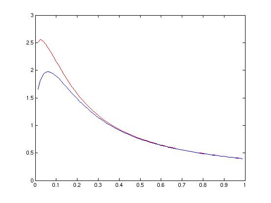
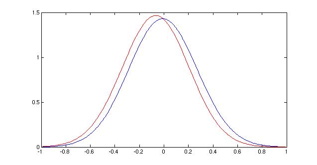
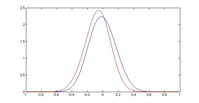
Once I decided to use parzen windows as my classification method, I settled on an h value of 0.0625. This value split the difference of the peaks of the two Evidence curves, and it also seemed to be on the same "scale" as the data, graphically. Larger values only showed two very smooth distributions right next to each other, whereas smaller values (not shown) were too bumpy to be useful because they overfit the data. The value chosen resulted in a smooth curve that also began to show differences in the shape of the distributions of the classes.
 |
 |
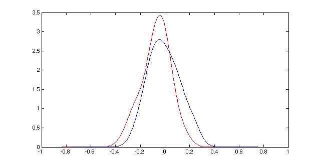 |
| Parzen window density functions for different choices of h. 0.25 (top), 0.125 (middle), 0.0625 (bottom) |
| Classification results on training data: | |
| Agreeing parties classified correctly / incorrectly | 10, 18, 36% |
| Opposing parties classified correctly / incorrectly | 36, 5, 88% |
| Total parties classified correctly / incorrectly | 46, 23, 67% |
| Classification results on testing data: | |
| Agreeing parties classified correctly / incorrectly | 7, 18, 28% |
| Opposing parties classified correctly / incorrectly | 38, 9, 81% |
| Total parties classified correctly / incorrectly | 45, 27, 63% |
Unsatisfied with this result, I decided to see if adding dimensionality would improve the discriminability of the classes. I reasoned that the different styles of pre-processing would be capturing different information about the data, and so by combin ing the different types of data available, I would hopefully see distinct clusters. To create two-dimensional vectors, I selected two styles of pre-processing, and then put the correlations resulting from the pre-processing into vectors. I found that the best combination was the correlations from data that had been smoothed with a window of width 3, and the same data, after it had been compressed. The classification results for this combination of features is highlighted in the table below
| (window width = 3) | Parzen, h = 0.25 | Parzen, h = 0.125 | Parzen, h = 0.0625 | KNN, k = 2 | KNN, k = 4 | KNN, k = 20 |
| Compressed vs Interference |
19, 10 20, 22 39, 32 |
19, 10 20, 22 39, 32 |
19, 10 20, 22 39, 32 |
1, 28 33, 9 34, 37 |
4, 25 35, 7 39, 32 |
18, 11 24, 18 42, 29 |
| Compressed vs Windowed |
19, 10 23, 19 42, 29 |
19, 10 23, 19 42, 29 |
19, 10 23, 19 42, 29 |
4, 25 26, 16 30, 41 |
21, 8 8, 34 29, 42 |
10, 19 31, 11 41, 30 |
| Windowed vs Interference |
20, 9 18, 24 38, 33 |
20, 9 19, 23 39, 32 |
20, 9 19, 23 39, 32 |
3, 26 28, 14 31, 40 |
15, 14 16, 26 31, 40 |
10, 19 28, 14 38, 33 |
After the poor showing by General Linear Discriminants on the 1D data, I chose to only experiment with K nearest neighbors and parzen windows on the 2D data. As in the 1 dimensional case, I selected the combination of features by looking for consistent ly good performance across classifiers.
The evidence curves and density functions in 2D took prohibitively long to compute, and so I tried a small number of values, and I found, again, that Parzen windows was best suited to the data, and gave the most consistent performance for different val ues of h. I then fixed h at 0.0625, as before.
| Classification results on training data: | |
| Agreeing parties classified correctly / incorrectly | 19, 10, 66% |
| Opposing parties classified correctly / incorrectly | 23, 19, 55% |
| Total parties classified correctly / incorrectly | 42, 29, 59% |
| Classification results on testing data: | |
| Agreeing parties classified correctly / incorrectly | 13, 13, 50% |
| Opposing parties classified correctly / incorrectly | 32, 16, 67% |
| Total parties classified correctly / incorrectly | 42, 32, 57% |
Discriminability is in fine detail. Methods that tried to smooth out fine detail made discriminability worse.
Does the way that people speak at the same time (or approximately the same time) yield information about alliances? No.
Conversation subjects were very dry.
People were very polite. (generally, did not talk at the same time.)
Not enough information captured about personality -- some people are just more likely to interrupt, whether or not they agree.
Many different styles of supporting / opposing each other:
 |  |  |
| In this conversation, person 1 and 2 (the leftmost speakers) are allied with the rightmost speakers. However, it seems like person 1 and 3 speak at about the same time, while person 2 and 4 speak at the same time. The groups rarely mix. | In this conversation, the leftmost 3 speakers are allied against the rightmost speaker. There seems to be a leader, who speaks opposite the opponent, while the other two chime in occassionally. | This convers ation is also has the leftmost 3 speakers allied against the rightmost speaker, but here, all three allies seem to take more equal turns. |