The Effect of Feature Selection on Classification of High Dimensional Data

MAS.622J

Fall 2006

Meredith Gerber

1. Problem

The Differential Mobility Spectrometer (DMS) is a promising technology for differentiating biochemical samples outside of a lab setting, but it is still emerging and analysis techniques are not yet standardized.

The DMS is a micromachined device that separates compounds based on the difference in their mobilities at high and low electric fields (Miller, Eiceman et al. 2000). (See Figure 1.)

Figure 1. Mode of DMS detection. Chemical separation in the DMS is achieved due to an alternating electric

field that is transverse to the direction of carrier gas flow. Changes in the DC compensation voltage allow

different compounds to pass through to the detector according to differences in mobilities between the high

and low fields. Image from (Krylova, Krylov et al. 2003).

The DMS has been used in laboratory settings for differentiating biologically-relevant chemical samples (Shnayderman, Mansfield et al. 2005), demonstrating that different bacteria, and even different growth phases of the same bacteria have distinct chemical characteristics that the DMS can detect.

DMS technology has even been applied in non-laboratory settings demonstrating its potential as a compact, reagent-less, fieldable sensor technology (Snyder, Dworzanski et al. 2004).

Analysis of this data is particularly challenging for two reasons:

1) The high dimensional nature of the data

2) The difficult link between identifiable data features and specific chemical compounds

Shown here are potential directions and points of consideration for pattern recognition problems involving high-dimensional data, with an eye towards selecting features with clear chemical relevance from high-dimensional data.

2. Data

The entire data set consists of 100 samples in each of three different classes corresponding to the material sampled: Bovine Serum Albumin (BSA), Ovalbumin (OVA), and water. Data were split into a training/testing subset (90%) and a sequestered validation subset (10%) randomly. In the training/testing subset of the data there were 85 BSA samples, 92 OVA samples, and 93 water samples. The training/testing set will be used to optimize parameters and feature sets, and the validation set will be used to validate parameters and selected features.

Each file has 98,000 dimensions corresponding to unique combinations of three different variables: scan number, compensation voltage (Vc), and polarity. When the positive and negative spectra are placed next to each other (even though they are recorded at the same time), each data file can be thought of as a matrix, the entries of which vary in two dimensions, uniquely, according to the chemical composition of the sample. (See Figure 2.)

B

A

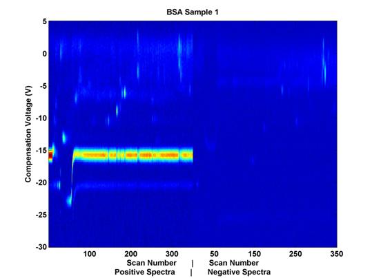
Figure 2. Example Data Sample. Compensation voltage is on the vertical axis and scan number (elution time)

is on the horizontal axis. The positive and negative spectra are placed next to each other horizontally,

for visualization purposes, but as their scan numbers indicate, the data were collected simultaneously.

(A) indicates the Reactant Ion Potential (RIP), and (B) indicates some chemical features which may be of

interest from a classification perspective as well.

The color represents sensor output values; the noticeable horizontal line (A) at compensation voltage -15 is the Reactant Ion Potential (RIP). It is mostly an artifact of the carrier gas with which the sample travels through the system. It is not hypothesized to yield relevant chemical data. The activity of interest seems to occur at compensation voltages of -14 and higher. These data have already been trimmed for relevance in the time domain, but an additional trimming here in the voltage domain could be beneficial in that it will help to remove from consideration nearly half of the remaining features.

All of the data have been pre-processed prior to this analysis. They have been trimmed in the time domain in addition to having been background-adjusted so that the baseline value is common across all samples.

The biggest pattern recognition problem here is the curse of dimensionality. The dimensionality of each sample is about 98,000 and there are 100 samples per class. The challenge is to create a system/classifier that given an input can determine the underlying class of that input--i.e., diseased or not diseased, with accuracy, given limited space/memory and limited time. This is a problem that is common in different biology applications (such as DMS, mass spectrometry, and microarray analysis).

3. Approaches

Feature selection has been performed on the training/testing data set so far with two approaches:

1. Two-class Fisher Linear Discriminant

2. PCA

In all cases, 50 features were selected from the data, and classification was performed with a range of numbers of features, between 1 and 50, to demonstrate trends in classification as the number of features used is changed. Additionally, features were selected at a range of radial distances from previously selected features (measured in scan-Vc space pixels). This was done to decrease the degree of correlation between selected features. The specific numbers of features and radial distances were:

Number of features used: [1 3 5 10 20 30 50]

Radial distances used: [1 2 3 5 8 10]

Classification has been performed with SVM (polynomial kernel) and K-Nearest Neighbors (K-NN) with a range of values for K:

Values for K: [1 3 7 11]

3.1 Fisher Discriminant, Two-Class (FLD)

For each pixel, the Fisher Linear Discriminant was calculated as indicated in Equation 1 (Duda, Hart et al. 2001). Pixels were considered as potential features and the features with the highest discriminant values were retained.

(1)

Where μ represents the mean of the pixel values across all samples and σ² is the variance of the values. The maximum values were between 1 and 1.5 and the range of values can be seen in Figure 3.

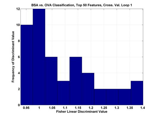
Figure 3. Histogram of the top 50 Fisher Linear Discriminant values. In the first cross-validation loop of the two

class comparison between BSA and OVA. The higher the discriminant value, the more separable the two classes.

The features with the highest Fisher Linear Discriminants are sent to the classifier for classification. However, in many cases, these features are not independent. Each pixel is a potential feature, but as can be seen in Figure 2, chemical features encompass a range of scans and compensation voltages. Potential features which are near to each other (in scan number and compensation voltage) are more likely to be correlated (in their information content). For this reason, beyond the two-class FLD, a radius restriction measure was implemented forcing selected features to be a certain radial distance (in scan-compensation voltage space) from previously selected features. A range of radius values were used between 1 (no restriction) and 10. As can be seen in Figure 4, features chosen with no radius restriction tended to be grouped together. These groups likely correspond to single chemical features in the signal. With a restriction radius of three (see Figure 5), there was still some grouping around chemical features, but additional chemical feature groups were included. Whereas with no restriction 50 features were in 5 groups, with a radius of three there were about 14 groups. With a radius of 10 (see Figure 6) there are about as many groups as features, but the quality of the features becomes more questionable. With such a large radius, the FLD value of the last chosen features becomes quite low, and anecdotally, some features appear more as though they are in a background portion of the signal.

Figure 6. Top 50 FLD feature locations with 10 unit restriction on feature location. Features were drawn

from the entire spectral set show (both positive and negative), across all scans and compensation voltages,

but were forced to be at least three units apart in the resolution of the scan-compensation voltage space.

3.2 Principal Component Analysis (PCA)

A dimension reduction approach was implemented using PCA. Rather than selecting specific pre-existing features, PCA extracts features from the original data, making linear combinations of potential features resulting in a feature set with lower dimensionality than the original feature set. In this case, however, features with clear chemical identity were desired, so a traditional PCA approach was modified to create a feature selector that would yield specific (scan number, Vc) points.

The eigen-decompisition step of PCA is space/memory intensive. In order to make this feasible, the dimensionality of the data had to be further reduced prior to feature selection. First, a subset of the data was selected in scan-Vc space (see Figure 7). Then, further reduction was achieved by down-sampling this space until fewer than 5,000 dimensions remained (out of an original 98,000.

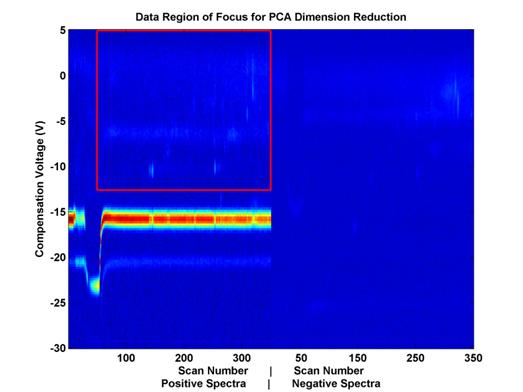
Figure 7. Feature space covered by PCA analysis. This space includes about 21,000 out of 98,000

potential features from the data displayed. This number of potential features had to be further reduced

in order to perform PCA because of space and memory constraints. To further reduce the potential

number of features, this space was evenly sampled.

Because chemically-relevant features were desired, PCA results were used as a means to select specific (scan, compensation voltage) coordinates as features. The majority of the variance was explained by one eigenvalue (see Figure 8). The top-ranked eigenvalue/eigenvector pair explained 70 percent of the variance, and the second pair explained only slightly more than 3 percent of the variance. Due to this, only the eigenvector coefficients from the first pair were used for feature selection (see Figure 9). However, because there are still almost 5,000 coefficients, only the top coefficients were used. Features were selected corresponding to the magnitude of the coefficients in this eigenvector. Features, generally came from the five different groups (A, B, C, D, and E, see Figure 9), but were not specifically forced to be distributed among these groups.

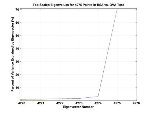
Figure 8. Percent of variance explained by top several eigenvectors. The top eigenvector explains

a bit over 70% of the variance whereas the second eigenvector only accounts for slightly more than 3%

of the variance.

E

D

C

B

A

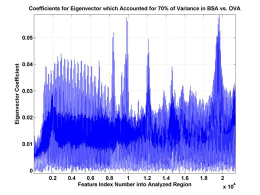
Figure 9. Eigenvector coefficients for top eigenvector. These coefficients explain 70% of the

variance of the distribution of (training and test) data. Some sets of high coefficient feature

indices are consecutive (A,B,C,D) while another has a sinusoidal nature (E). This likely indicates

features which are either more oriented along the scan- or Vc-axes.

3.3 Sequential Forward Selection (SFS)

Sequential forward selection was implemented using a correlation coefficient-based objective function. Sequential forward selection chooses features one at a time, at each point, finding the next feature that maximizes the objective function with respect to that potential feature and the previously chosen features (Gutierrez-Osuna). This has the disadvantage of needing to compute the objective function result for each of the tens of thousands of potential new features, in addition to the disadvantage that once a feature is added, it cannot be removed. (Subsequent instantiations of this feature selection technique such as Plus-L Minus-R Selection and Sequential Forward Floating Selection begin to address the second disadvantage listed previously.) The advantage of this method is that information regarding how a new feature would interact with the already chosen group is considered.

Because a calculation is made for each potential feature, the processing time required by this algorithm is tremendous. Due to time and space concerns, this algorithm was limited in the scope of the features it could consider, similar to PCA, as described above. Specifically, the physical extent of the features was limited to those in the red box in Figure 7, and that space was further down sampled to limit the number of features considered to be no more than 5000.

The objective function used in this case is illustrated below in equation 2.

(2)

Where Y_M is the feature set with M features, ρ_ij is the correlation between features i and j, and ρ_ic is the correlation between feature i and the class labels, c. At each choice to add another feature, this technique should choose the feature that maximizes the sum of the correlations between the class labels and each feature individually while minimizing the sum of the correlations between all combinations of features chosen. So, a feature which is more highly correlated with class labels is more likely to be chosen, and a feature which is less correlated with already selected features is more likely to be chosen. The objective function value should increase as features are selected which are correlated with class labels but not with each other, and then decrease, as subsequent features are either less correlated with class labels or more correlated with previously chosen features. In the BSA vs. OVA comparison task, the objective function values evolved as is shown in Figure 10.

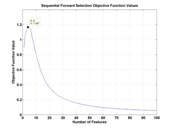
Figure 10. Objective function values for Sequential Forward Selection in BSA vs. OVA. The peak of this

curve is marked and occurs at 4 features.

In this method of feature selection, the ideal feature set would be that represented by the peak of the objective function. As can be seen in the results section below, for the sake of consistency, classification has been performed for a consistent number of features across all techniques, in this case, going far beyond the peak here at four features. See section 4.3 for results. It is interesting to note that the drop off in performance as demonstrated by the objective function is drastic, seeming to indicate that classification performance with 20 or more features may be worse than performance with one feature. In reality, this would depend on the size of the training set data and the nature of the classifier.

4. Results and Discussion

The results shown here represent 4-fold cross-validation results on the training/testing subset of the data. Each feature selection method was used to select 50 features under a range of radius restriction rules as described earlier. Results for a specific binary comparison, feature selection method, and classification method are shown in each plot. Percent correct classification is shown as a function of both the number of features selected and submitted to the classifier and the radius restriction that was implemented. A radius restriction of one (the blue diamond) is the same as making no restriction on feature location. The baseline level of comparison for these binary tests is 50% correct classification, the bottom of the vertical scale shown here. Black error bars have been used here to demonstrate the variance around each point across the four cross-validation folds. In most cases, the variance was less than 1% and the error bars cannot be seen. In all cases, classification was performed with Support Vector Machines (SVM) in addition to K-Nearest Neighbors (K-NN) with a range of K values. Note that for each classification task within a particular feature selection technique, the sets of features submitted to the classifiers were the same. That is, the feature set was determined by the parameters relating to the feature selection technique, the number of features, and the radius restriction rule, but not by the classifier itself. Therefore, all comparisons within a classification task between classifiers, are direct comparisons.

4.1 FLD

The two-class Fisher Linear Discriminant was calculated for each potential feature (scan-compensation voltage point) independently and the features with the top FLD values were chosen, as detailed above. Some interesting trends can be seen in Figure 11 and Figure 12 which document classification results for the SVM and K-NN, K=7 classifiers, respectively. First, both classifiers demonstrate a great ability to discriminate between water and BSA, with typical results above 90% correct classification and the highest results above 95% correct classification. Second, for both classifiers, the accuracy shows a slight increase as additional features are added but stops increasing or even decreases after a certain number of features is exceeded. This is likely due to overfitting, because with 50 features, the classifier might be making a 50-dimensional decision boundary, but this is really only a two-class decision. In the case of the SVM classifier, the lower performance, or the inability to improve performance with the additional features may also be due to a relative lack of training data. As the dimensionality of the decision space (corresponding to the number of features used) increases, the concentration of training points in that space decreases making the calculation of a specific decision boundary more difficult. This is related to the first issue in that the sparsely populated decision space will be more likely to precipitate a boundary that crosses a dimension where the training data for the two classes happen to be different, but that in reality is not relevant to the decision at hand. More recent feature selection methods have tried to address this question by applying false discovery rate controlling methodologies from the statistical fields (Reiner, Yekutieli et al. 2003). Third, higher radius restriction leads to equal or higher classification results, to a point. This is especially evident in the SVM results of classification with 30 features. As can be seen there, with the exception of the highest radius restriction rule, the classification percentage is according to the radius restriction rule; that is, the features selected with no restriction performed the worst (about 88%) and the feature selected with an enforced distance of 8 between the features performed the best (about 98%). In the K-NN results the differences are not as extreme, but it is clear that the feature set selected without any restriction does not perform as well as the others. It should be clear that this benefit in performance comes with minimal added cost in processing time since the calculations necessary depend only on the features already selected as opposed to the features which could be selected. In a high-dimensional data set, or one with many, many potential features, this is extremely significant. While methods which compute the interaction of selected features and classification abilities of entire subsets (rather than individual features) may yield more accurate results, this method of selecting features in part based on location in order to reduce correlation in the feature set delivers a lot of classification ‘bang’ for the processing ‘buck’.

Figure 11. Classification Performance for Water vs. BSA (SVM) FLD feature selection. Note that classification

improves as features are added, until about 30 features. Also, note that classification at this point is generally

better with a higher radius rule, likely because selected features are not as correlated.

Figure 12. Classification Performance for Water vs. BSA (K-NN, K=7) FLD feature selection. Note that

performance and trends are generally to similar to those with SVM (see Figure 11). Classification improves as features

are added, until about 30 features. Also, note that classification at this point is generally better with a higher radius

rule, likely because selected features are not as correlated.

A summary of the results from FLD feature selection for all classification tasks can be see in Table 1. Unsurprisingly, the classifiers performed better on the tasks distinguishing between protein and water than on the classification task distinguishing between one protein and another protein. Over the range of parameters tested here, the performance of the K-NN classifier and the SVM classifier were similar in the last classification task, though, here, for this particular subset of parameters, the K-NN classifier performed better.

Summary of FLD classification results
At r=3, 30 features

Comparison	SVM	K-NN, K=7
H2O vs. BSA	93%	94%
H2O vs. OVA	96%	95%
BSA vs. OVA	83%	88%

Table 1. Classification Performance Summary for FLD feature selection. These are results of classification with 4-fold

cross-validation on the training/testing data set. The K=7 K-NN classifier was chosen as a point of comparison for

the SVM results.

4.2 PCA

The vector coefficients of the first principal component of the test data were used to rank potential features and select the top 50 features as detailed above. Interestingly, the top coefficients did not have the same discrimination ability as those chosen by FLD (the performance was worse), though after the addition of fifty features, the performance was nearly comparable (see Figure 13). Further, the trends evident in the FLD results, are not as evident in the PCA results. First, the ability to discriminate between protein and water is good but not great, with results between 85% and 90% correct classification (see Table 2). This is in contrast to FLD results above 90%. Second, the classification success increases as features are added without indicating a leveling-off, much less, a decrease in classification rate. This is also the case for the SVM classifier in this classification task. In the other classification tasks, the general trend was increased performance with increased number of features and a leveling off after 30 features was the exception to the rule. Third, there does not appear to be an affect of radius restriction rule on K-NN classification with the PCA selected features. With FLD, some effect was observable with K-NN classification, but it was stronger with SVM classification. Here, too, SVM classification demonstrates a trend more readily than K-NN, though it is not as clear as with the FLD selected features. In particular with K-NN, it seems that number of features has a greater impact on classification result than radius restriction enforced. It is interesting to see that the K-NN ‘decision boundary’ does not seem to become less robust as there are an increasing number of dimensions across which to calculate the nearest neighbors, but not an increasing number of training data available to populate the decision space.

Figure 13. Classification Performance for Water vs. BSA (K-NN, K=7), PCA feature selection. Compare to results

with FLD feature selection (Figure 12). Trends are similar, though classification accuracy is not as good, in comparison.

A summary of the results of classification for all three classification tasks using features dictated by PCA can be seen in Table 2. Interestingly, the results for the tasks comparing water and protein are not as different from the protein-protein comparison results as with FLD feature selection. Classification on the PCA-selected features in the protein-protein task did just about as well as with FLD-selected features in the same tasks, but the water-protein classification results are lower than with FLD.

Summary of PCA classification results
At r=3, 30 features

Comparison	SVM	K-NN, K=7
H2O vs. BSA	88%	90%
H2O vs. OVA	84%	88%
BSA vs. OVA	85%	86%

Table 2. Classification Performance Summary for PCA feature selection. These are results of classification with 4-fold

cross-validation on the training/testing data set. The K=7 K-NN classifier was chosen as a point of comparison for

the SVM results.

4.3 SFS

Sequential Forward Selection was implemented with a correlation coefficient-based objective function, as detailed above. It is important to note that of all of the techniques implemented, SFS took the most processor time, by far. Results that took other feature selection classification scripts on the order of 20 minutes to complete took this feature selection classification script on the order 10 hours to complete. Due to processing time necessary, this may not be a viable alternative for high-dimensional data sets, unless time is really not an issue. That being said, the trends that resulted from SFS feature selection would not recommend it in any case. Because they are so different, they are discussed outside of the framework of the previous two feature selection methods. Classification performance from the Sequential Forward Selection based features was dismal, barley above, and sometimes below the baseline performance of 50% that would be expected with random class assignments. For all classifiers, no trend was observed with respect to radius restriction rule. The trends observed with respect to the number of features used were unique and merit further discussion. In classification with SVM (see Figure 14), classification performance was extremely low for all numbers of features (below 60%), but worse for 20 or more features, and decreasing as the number of features were added beyond 10. In classifying the data based on the same feature set using K-NN, K=1 (Figure 15) the results were above 90% for one feature, but decreasing and below 60% for all other numbers of features. In the K-NN, K=7 classifier (Figure 16), the same feature sets were classified with a more familiar trend of improving classification rates as more features are added between 0 and 10 features and decreasing classification rates as features are added beyond 20 features. However, the maximum classification rate here is about 63% at 10 features and the results are below 60% for 1, 3, 30, and 50 features. In part, this trend may indicate the ability of the SFS algorithm to choose a good initial feature but that subsequent features do not provide information that is ‘good’ for the purpose of these classifiers. The first feature may indeed be good despite the low SVM performance, because, as it has been observed in the past, SVM does not perform as well with 1 feature as it does with 5 to 10 features. Further the first feature which SFS selected as having the best correlation with the class labels may have relatively low signal strength/amplitude, so that it is easily drowned out when the dimensionality of the feature space is increased to accommodate other features with lower correlation but higher signal. This explanation does not immediately clarify why the performance of the K-NN, K=7 classifier was so much less than the K-NN, K=1 classifier for 1 feature, and this remains a point of further investigation.

Figure 14. Classification Performance for Water vs. BSA (SVM), SFS feature selection. Compare to results with FLD

feature selection (Figure 11) and SFS objective function value trend (Figure 10).

Figure 15. Classification Performance for Water vs. BSA (K-NN, K=1), SFS feature selection. Compare to results with SVM

classification (Figure 14) and K-NN classification, K=7 (Figure 16).

Figure 16. Classification Performance for Water vs. BSA (K-NN, K=7), SFS feature selection. Compare to results

with FLD feature selection (Figure 12) and PCA feature selection (Figure 13).

A summary of the results of classification results with the SFS-selected features can be seen in Table 3. Generally, it seems as though the features selected did permit classification between protein and water somewhat better than the baseline (around 60%) while classification between the two protein classes was not achievable with the K-NN classifier and was minimally achievable with SVM.

Summary of SFS classification results
At r=3, 30 features

Comparison	SVM	K-NN, K=7
H2O vs. BSA	57%	59%
H2O vs. OVA	63%	63%
BSA vs. OVA	57%	46%

Table 3. Classification Performance Summary for SFS feature selection. These are results of classification with 4-fold

cross-validation on the training/testing data set. The K=7 K-NN classifier was chosen as a point of comparison for

the SVM results and for results of other feature selection methods.

Overall, it is interesting to note that the feature selection method that took the most investment in terms of processor time yielded in fact the worse results, indicating in a cautionary way, that methods which seem like they may be the most comprehensive in some ways are not guaranteed to perform the best unless it is clear that they are explicitly the best for the data to be classified. Further, it is possible to use somewhat naïve models of feature distribution in forming selection techniques that are both reasonably fast and effective (like the radius restriction rule discussed here).

6. Acknowledgements

I would like to gratefully acknowledge Mindy Tupper at the Charles Stark Draper Laboratory who oversaw the collection of this dataset.

7. References

Duda, R. O., P. E. Hart, et al. (2001). Pattern Classification, John Wiley & Sons.

Gutierrez-Osuna, R. Introduction to Pattern Analysis, Texas A&M University.

Krylova, N. S., E. Krylov, et al. (2003). "Effect of Moisture on the Field Dependence of Mobility for Gas-Phase Ions of Organophosphorus Compounds at Atmospheric Pressure with Field Asymmetric Ion Mobility Spectrometry." Journal of Physical Chemistry A 107: 3648-3654.

Miller, R. A., G. A. Eiceman, et al. (2000). "A novel micromachined high-field asymmetric waveform-ion mobility spectrometer." Sensors and Actuators B 67: 300-306.

Reiner, A., D. Yekutieli, et al. (2003). "Identifying differentially expressed genes using false discovery rate controlling procedures." Bioinformatics 19(3): 368-375.

Shnayderman, M., B. Mansfield, et al. (2005). "Species-specific bacteria identification using differential mobility spectrometry and bioinformatics pattern recognition." Anal Chem 77(18): 5930-7.

Snyder, A. P., J. P. Dworzanski, et al. (2004). "Correlation of mass spectrometry identified bacterial biomarkers from a fielded pyrolysis-gas chromatography- ion mobility spectrometry biodetector with the microbiological gram stain classification scheme." Analytical Chemistry 76: 6492-6499.