Graphical Models, Bayesian Networks

Background

Probabilistic graphical models are powerful modeling tools that provide a natural representation for different problem domains that have inherent uncertainty. These models support the use of efficient algorithms that allow for automatic construction and query answering [1,2], helping in the reasoning and decision making process on the subject under analysis.  In our application, we focus on the use of Bayesian networks to help us find the most probable explanation for the observed evidence on the funded (or not) listings dataset given by a selected feature set. Bayesian networks are defined as causal networks (with the strength of the causal links represented as conditional probabilities obtained from estimation methods) using a complete testing information data set.

Goal

Based on a sampled dataset of Prosper® listings ,  develop a series of Bayesian network models that can assist to discriminate  listings that were fully funded from those which closed unfunded.

Methods

From the set of the”FS96” feature set, the best nine features that explain the variation of the data (based on previous PCA analysis) were selected. These features were employed to generate several Bayesian graphical model structures which aim to best explain the observed data and represent the causal relationship between the information variables. In addition, these models provide a probabilistic reasoning framework to determine how likely it is for a listing to get funded or not.

The purpose of organizing a Bayesian network model is to give estimates of certainties of events that are not directly observable [2]. This the context of our application, we would like to obtain a posteriori probabilities of a listing getting funded or not given the observed states from a set of discrete information variables.  The purpose of this is to use the Bayesian network as a classification tool and evaluate its performance on the complete sampled dataset. In addition, the Bayesian networks can be employed as a decision tool, providing the estimates of certainties of the listing getting funded or not given some observed states.  For example, we can ask queries of the form:

• What’s the probability of getting a listing funded if the debt to income  ratio is low, the maximum borrower’s rate is high, there is a low amount requested, and there is no endorsement?
• What is the probability of a listing getting funded if there are the credit grade is average the amount requested is high and the amount delinquent is low and open credit lines are low?

Training and Testing Dataset

The dataset contained 10,000 samples of listings that were funded and 10, 000 samples of listings that closed unfunded. The stratified sampling to obtain these sets is described in the Classification section under Feature Selection. The complete sampled dataset included all observations for the selected features in each of the two classes (listings funded and not funded). Considering the effect of accounting for prior probabilities we trained each of the Bayesian network models with 90% of the dataset in order to estimate the parameters (conditional probability tables) and remaining 10% of the dataset was employed to test the models as classification tools. We performed testing over 10 iterations of holdout data (taking into account the variation between the created models).

Variables and Description

The ten quantized features used as variables for the Bayesian networks are:

1. Amount Delinquent
2. Open Credit Lines
3. Amount Requested
4. Borrower’s Max Rate
5. Credit Grade
6. Debt to Income Ratio
7. ‘Good Candidate’ Descriptor
8. Funding Option
9. Endorsement

12. Loan

The descriptions for each of the feature variables are defined next. Each of the variables was discretized based on their independent frequency histogram over the whole sampled dataset.

Information Variables

1. Amount Delinquent: The monetary amount delinquent at the time this listing was created.
   Low: < 5000
   High: >5000

2. Open Credit Lines: Number of open credit lines at the time the listing was created.
   Low:  < 5
   Medium: (5, 10]
   High: >10
   
3. Amount Requested: The amount that the member requested to borrow in the listing.
   Low: <3000
   Moderate: (3000, 5000]
   High: (5000,10000]
   Very High: >10000
   
4. Borrower’s Maximum Rate: The maximum interest rate the borrower is willing to pay when the listing was created.
   Low: < 0.15
   Moderate: (0.15, 0.20]
   High: (0.20, 0.27]
   Very High: >0.27
   
5. Credit Grade: Credit grade of the borrower at the time the listing was created.
   Poor: < 560
   Average: (560,620]
   Good: (620, 680]
   Very good: >680
   
6. Debt to Income Ratio: The debt to income ratio of the borrower at the time the listing for this loan was created
   Low: < 2
   Medium: (2,6]
   High: > 6
   
   

   Binary Information Variables

   (states: True or False)

7. ‘Good Candidate’ Descriptor.  Text description used in a listing’s profile.
8. Funding Option.  The listing is open for it's duration.
9. Endorsement. Does the listing have an endorsement comment on the profile
   
   

   Hypothesis variable.

12. Loan. The listing posted is funded. (Does the loan get granted?)

Once the information and hypothesis variables have been defined, we need to establish the directed links for a causal network.

Methods

Learning the structure of the Bayesian Network

From training dataset we have the observed samples of cases from an assumed Bayesian network N over a universe U of directed acyclic graphs (DAG)*. Our work is to reconstruct the Bayesian network from these set of cases. This is precisely the framework to apply structural network techniques. In general, there is no assurance that these cases actually came from a “true” network, but this will be our assumption. Another assumption is that the set of samples is fair, which means that the set of D cases in the training data reflect the distribution PN(U) which is determined by N. For the structural learning techniques described below we assume that all links in N are essential.  The task then is to find a Bayesian network M that closely resembles N.

Tools.- In order to implement the different structural learning algorithms as well as the parameter estimations for each of the proposed Bayesian networks two main tools were employed in addition to self -created code.

1. Kevin Murphy’s Bayes Net Toolbox
2. Philippe Leray & Olivier Francois BNT Structure Learning

Exhaustive Search and PC algorithm

In principle, if we can perform parameter learning for all possible structures and then select those models for which PM(U) is as close to PD(U) as possible. This approach is an exhaustive search over an extremely large set of Bayesian network structures. The algorithm that was implemented to try to perform this search is the PC algorithm as described in [2, pg.235]. The number of different structures  r(n) grows super-exponentially with the number of  n as described by:

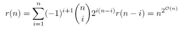
With the 10 nodes that we have as a basis for our Bayesian networks, there exist 4.2 x 1018  different directed acyclic graphs that can be generated.

The main problem when implementing the exhaustive search algorithm was ran over the sampled training dataset the computer suffered from overflow and was not able to converge. Empirically when the number of nodes is larger than 4 this algorithm will not necessarily converge. In the case of converging there exist other two problems:

1. The end results of trying the algorithm can produce several good candidate models that may not necessarily have good classification performance
2. The selected model can have a very close representation of  PD(U), but we can be overfitting the data.

Looking for another option to learn the structure of the Bayesian network, we tried the PC algorithm. This is a constraint-based technique that tries to learn the model that best represent the data by establishing a set of conditional independence statements between the features and  using this set to build a network with d-separation properties corresponding to the different conditional independences. The conditional independence tests were conducted by implementing  chi –square tests on the feature set.

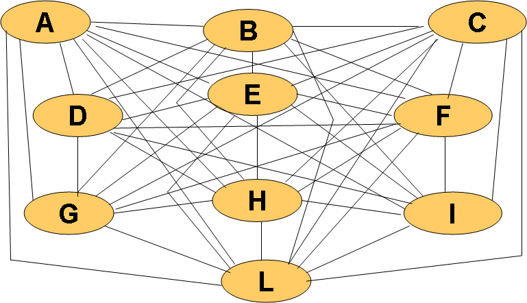
The starting graph for the PC algorithm, where all of the features are interconnected in a non-directed structure.

When implementing the PC algorithm, the results did not converge to a single graph. A possible cause if this is when the algorithm encounters uncertain regions, in which you cannot direct the links due to a removal  of other links based on the independence tests. The limitation of the use of this algorithm is the assumption that there are no hidden variables that can obscure the causal relation between the variables in the Bayesian network. It is important to mention that even a correct statistical test for independence may not provide the correct d-separation properties (even in a large dataset), which means that the conditional probabilities in the network may hide some dependencies [1].

Markov Chain Monte Carlo Method

The goal of structure learning is to look for a Bayesian network structure that can represent the database as well as possible and is not very complex. In the previous section we proposed how to perform structural learning based on independence tests and in this section we focus on score-based learning, particularly the Markov Chain Monte Carlo method (MCMC).

In general, score-based learning gives certain score to each of the Bayes net structures. This score gives a sense of how likely it is for the structure to generate the observed dataset. The simple notion is to look for a structure that provides the best score. The way to look for each structure is specified by a searching procedure.

The score function used to evaluate each network was the Bayesian Information Criterion (BIC). This function provides a score that takes into account how well the data fits the model as well as how complex the model is.

In order to search the space of the different Directed Acyclic Graphs (DAG’s) se used the structural learning tool to implement an MCMC algorithm [3,4]. The input for this algorithm was the value of each case (sample) for each one of the nodes (variables) from complete data set of all 10 observed features (this method is not deterministic). For this algorithm the hypothesis variable was not initialized to be a consequence of the information variables. Without the initialization, the produced output gives a more general structure of how all of the variables represent the observed data, provided that Loan can be a parent and son of other variables. The reason not to initialize the Loan variable is to use the network mostly as a classification tool and improve its performance over the testing data.

After running the MCMC algorithm over the complete observed dataset we obtain the following Bayesian network.

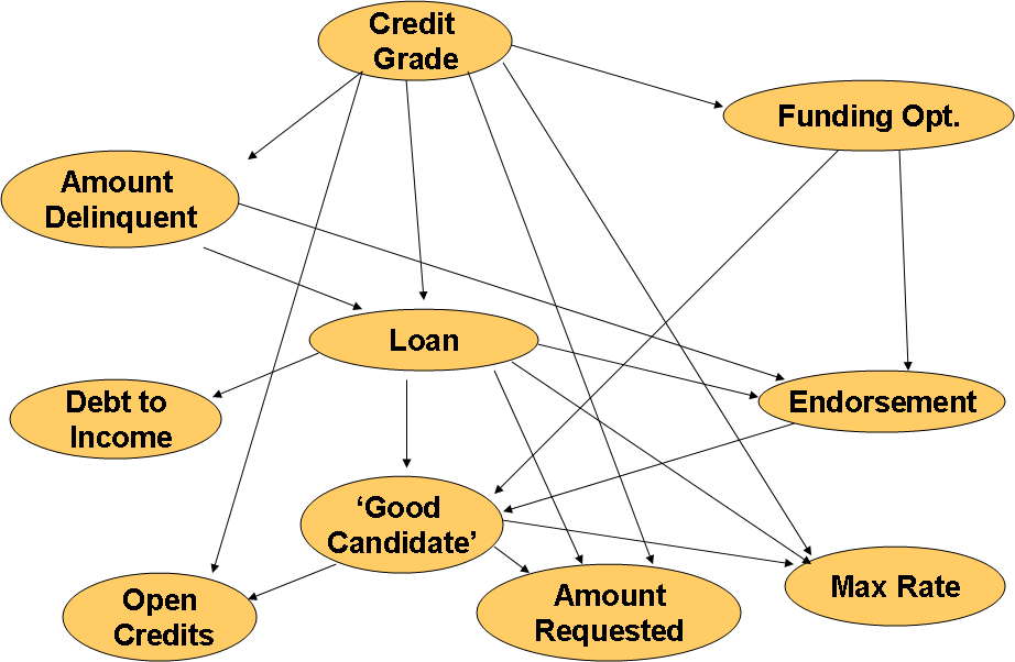
From this model we can observe that the Loan variable has a causal relationship to the Credit Grade and Amount Delinquent variables, and is a parent of Debt To Income Ratio and Borrower’s Maximum Rate. Is interesting how this model captured these major relationships, however, intuitively we would like to have Loan to be a hypothesis variable and not be a parent of the other features. The reason for this is so we can use the same model can for classification as well as for decision assistance over the certainties of getting a listing funded or not, given the states of the observed variables. The evaluation of this model as a classification tool (including is BIC score) is presented in the results section.

Chow-Liu Trees & K2

When using the Bayesian Information Criterion score we incorporate a penalty term that tries to reduce the model’s complexity. Another methodology that allow for a reduced complexity model is to restrict the types of network structures. One of this type of restrictions is to only allow a set of tree-shaped structures, namely Chow-Liu Trees. For this application we are initialiazing the type of DAG’s derived from the maximum weight spanning tree algorithm (MWST) proposed by Chow & Liu [5]. This method associates a weight to each edge. In this case the weight is the mutual information between the two variables. The result gives an undirected tree that can be oriented with a choice of a root. We then used the oriented tree from the MWST algorithm to generate an enumeration (topological) order initialization for the K2 learning algorithm. For our application the root that selected was the hypothesis variable: Loan (class node).

The goal of the K2 algorithm is to maximize the probability of the structure given the data. The size of the search space is reduced by the node order selected and choosing the root node. This algorithm makes the search space to a subspace of all the possible DAG’s that admit this order as a topological order selecting the class node as the end of the tree with no descendents. When using K2 algorithm the parents are tested in order to best upgrade the score metric (BIC). The input for this algorithm was the value of each case (sample) for each one of the nodes (variables) from complete data set of all 10 observed features (this method is not deterministic) as well as the node order that was generated by the MWST algorithm.

The Bayesian network generated by this problem is depicted in the following figure:

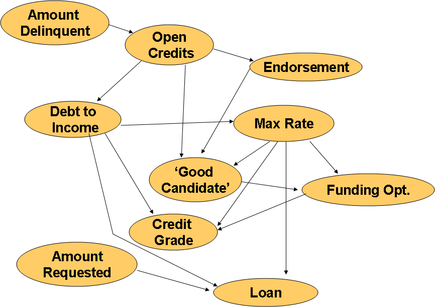
From this graph we can easily see that the main influence features on the a listing getting funded or not (Loan variable) are the Amount Requested, the Debt to Income Ratio and the Borrower’s Maximum Rate. This result is particularly interesting because it matches the results provided by the Principal Component Analysis & Linear Discriminant Classifiers that were described earlier for this project. Of particular interest is the fact that modeled not interpreted the Credit Grade a parent of any other variable. This interesting result mainly due to the fact that this algorithm is very sensitive to the topological order that uses as an input. The evaluation of this model as a classification tool (including is BIC score) is presented in the results section.

Parameter Estimation

For each of the Bayesian Network models, the parameters (conditional probability distributions) had to be estimated. In our application we are dealing with a complete dataset of all observed information variables. Assuming that we have a Bayesian network M = x (S, θ) with a structure S and parameters θ, and a set of data D, as all case samples of the observed variables. In order to make the estimation of the parameters of each model given the observed data set we performed a Maximum Likelihood estimation (MLE). With this method we obtain the conditional probabilities that maximize the probability of the dataset for a specific model.

Simple Bayesian Network

In order to provide a basis of comparison with the learned structures we proposed designing three other Bayesian Networks that included a simple Bayes net similar to a Naïve Bayes model, a Noisy-Or Bayes net and an empirical belief network. For each of these models we calculated the BIC score and estimated their parameters using MLE.

The Simple Bayes net structure was directly coded using Murphy’s toolbox [3]. This network has the following structure:

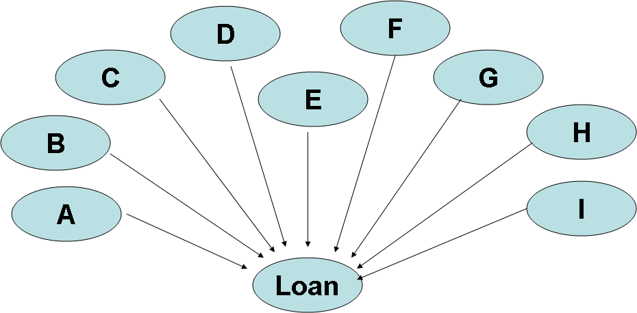
For this structure, all of the information variables are the parents of the hypothesis variable which describes the state of getting a Loan granted. The simplicity of this model can be deceiving, since the conditional probability table for the class variable is as large as the look-up table for the classification problem. One of the drawbacks of such structure is that it ignores any influences or causal descriptions among the information variables.

Noisy-Or Bayes Net

From the simple Bayes net structure described before, we concluded that the probabilities that take into account the state of the class node given each one of the states of the information variables become very small and in order to improve the performance of such network, we proposed divorcing the parents by directing certain parents to introduced mediating variables (Noisy functional dependence). This allows to cluster variables into sets and have the hypothesis variable be dependent on these new features.

The set of complimentary variables that were created in order to cluster the information features are: Listing Profile, Loan Risk and Member Support. These variables have also been discretized in the following manner.

• Profile. States: Poor, Average, Good
• Loan Risk: Low, Medium, High
• Member support: Low, Medium, High

With this new technique the network generated has the following structure:

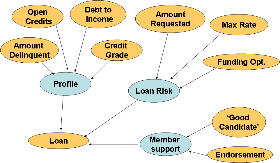
This network was directly coded into the Murphy’s toolbox [3], and its parameters were estimated with using MLE. When evaluated using the BIC scoring function and classification performance we obtained the same values that we obtained for the Naïve Bayes net. However, the computation time to evaluate this network was reduced in approximately 13%.

Empirical Belief Bayes Net

Based on our ‘expertise’ of the observed data (provided by the original descriptive statistics), we generated an empirical belief network, in order to contrast its performance results with the learned structures and the simplistic Naïve Bayes net. This network is depicted in the following figure:

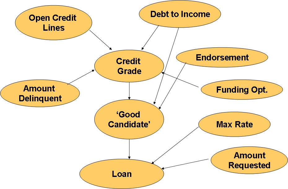
In this network we tried to capture the main influences of the Amount Requested and the Maximum Rate as independent features that affect the Loan variable. We tried to maintain the simplicity of the structure by assuming most of the features independent from each other and minimizing the influence among them. For this network the parameters were estimated using MLE using the training dataset of the sampled observations. The BIC score was calculated and compared its performance as a classification model with the other Bayesian network models.

Maximum A Posteriori Decision Rule (MAP)

In order to evaluate each of the proposed Bayesian network models as a classification tool, we employed a MAP decision rule, to calculate the probability of the listing getting funded or not (Loan = True or False), given each one of the sample cases of the testing data. This metric allowed us to see how well did each of the structures performed.

One the main problem to avoid is overfitting, that is, being able to generate a classifier that can correctly classify not-yet- seen cases. To address this problem we used different parts of the complete data set for training and testing as described earlier in the training and testing data set section.

Results and Discussion

The BIC score and the classification performance for each of the Bayes network structures is presented in the following table:

Bayesian Network	BIC score (x 10^5)	Classification Performance
Learned Structure (MCMC)	-1.33	0.76
Learned Structure (Chow-Liu Tree & K2)	-1.34	0.7525
Simple Bayesian Network	-1.83	0.7580
Empirical Belief Network	-1.42	0.5620

From these results we can observe that the network that best represents and classifies the observed data is the learned network using the MCMC algorithm. However, this network is hardly going to be used as a decision tool due to the fact that the Loan variable (class node) is a parent of other features and we require for this node to not have any descendants. A simpler learned model with the Chow-Liu Tree and K2 algorithm had very similar score and performance as the MCMC algorithm. The tradeoff between complexity and performance favors this model overall.

An very interesting result is the one obtained from the simple Bayes Net, which overall had the worst BIC score but one of the best performances in classification. This suggests that the BIC score and classification performance are not always in agreement, allowing us to have a network can be well used as a classification tool but that cannot totally represent the observed data. This is something that should be further analyzed and demonstrated.

The previous result is supported in a way by the values obtained for the empirical belief network, which had a very good BIC score but a terrible classification performance. These results suggest that our intuition on how the variables were related was more or less accurate (for this metric). In other words it can represent the observed data good enough but it cannot be used a classification tool, since its performance was slightly over 50%.

Future work

• Perform Optimal discretization of information variables
• Augment the Variable (Feature Vector) to try to capture the influence of other features to the outcome.
• Evaluate other Structure learning algorithms on a larger dataset and compare the classification performance
• Validate the models as decision tools comparing its decision performance with common bank specific tools

Main References

• [1] F. V. Jensen and T. D. Nielsen. "Bayesian Networks and Decision Graphs". Springer. 2007.
• [2] R.O. Duda, P.E. Hart, and D.G. Stork, “Pattern Classification”, New York: John Wiley & Sons, second edition, 2001.
• [3] Kevin Murphy’s Bayes Net Toolbox, 2001
• [4] Philippe Leray & Olivier Francois BNT Structure Learning, 2007
• [5] Chow, C. K. Liu, C. N. 1968. “Approximating discrete probability distributions with dependence trees”. IEEE Transactions on Information Theory, IT-14(3), 462-467.