Prediction of
Paroxysmal Atrial Fibrillation(PAF) Using HMM-Based Classifiers
Ghinwa Choueiter: gfc00@mit.edu
Brief Overview of the problem at hand: PAF
Atrial Fibrillation is a very common major cardiac arrythmia. Cardiac Arrythmia is a generalized term used to denote alteration of the heart’s rythms that disrupt the normal synchronized contraction sequence. Arrythmias can be usually recognized by evaluating the EKG in a systematic manner.
Briefly described, the heart
consists of four chambers, two upper chambers called the left and the right
atria and two lower chambers known as the right and left ventricles. In order
for the heart to pump, it must first receive some sort of electrical
stimulation that will cause the muscle to contract. The whole cycle of
electrical stimulation is known as normal sinus rhythm (NSR), which describes a
form of orchestrated synchrony between the atria and the ventricles of the
heart.![]() In the broadest sense, AF represents the
loss of synchrony between the atria and the ventricles. The atria depolarize
repeatedly and in an irregular uncontrolled manner usually at an atrial rate
greater than 350 beats per minute. As a result, there is no concerted
contraction of the atria. The chaotic atrial depolarization waves penetrate the
AV node in an irregular manner, resulting in irregular ventricular
contractions. The QRS complexes have normal shape, due to normal ventricular
conduction. However the RR intervals vary from beat to beat. For more info see
[8].
In the broadest sense, AF represents the
loss of synchrony between the atria and the ventricles. The atria depolarize
repeatedly and in an irregular uncontrolled manner usually at an atrial rate
greater than 350 beats per minute. As a result, there is no concerted
contraction of the atria. The chaotic atrial depolarization waves penetrate the
AV node in an irregular manner, resulting in irregular ventricular
contractions. The QRS complexes have normal shape, due to normal ventricular
conduction. However the RR intervals vary from beat to beat. For more info see
[8].
Paroxysmal AF (attack) occurs intermittently and varies in frequency and duration from a few seconds to more protracted episodes lasting several hours or even days.
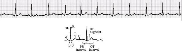
Figure –1 ECG
illustrating a normal sinus rhythm.
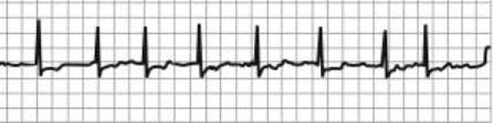
Figure –2 ECG illustrating a subject with atrial fibrillation
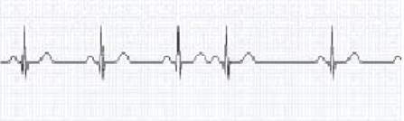
Figure –3 ECG
illustrating a heartbeat waveform with a premature beat, which might predict
the onset of a PAF
The aim of this tool is to attempt to solve two problems:
·
Detect whether a person has AF or not.
·
Predict whether a person with AF is about to have an
attack or not.
Description of the Data
The data originally consisted of two sets of 30-minutes double-channel records of ECG sample at 128 samples/sec. The number of recording in each set is 50 to be divided between training data and test data. The n-set comes from subjects confirmed with no PAF. The p-set comes from subjects who have paroxysmal atrial fibrillation (PAF). The p-set is itself divided into 2 where 25 of the recordings are for subjects with atrial fibrillation about to experience an episode of PAF and the rest do not. All the data is labeled so the training is supervised. Since the dataset was originally too large certain alterations were done in order to facilitate its manipulation:
· A single channel was used instead of 2.
· For certain problems, the data was down-sampled by 8.
· For certain problems, only a chunk of the whole recording was considered.
I do not claim that this is the best way to solve the problem of large data set. However, this is just a proposed solution also required due to the absence of a powerful machine on which the code could be run.
Features
From the description of the problem at hand, certain proposed features are the R-R intervals or the spectrogram of the heart signals. The R-R features were initially used with a simple HMM-based classifier but the recognition rates obtained were very low so the features were dismissed.
In order to preserve important information in the waveform such as the morphology and the interval timing, the features consisted simply of samples of a single ECG channel. The original records consisted of 230400 samples each but were down sampled to 28800 samples. Another set of features consisted of the cepstral coefficients.
Preprocessing
In certain cases of the ECG recordings some problematic sources might arise such as muscle noise and power-line interference causing signal characteristics especially the mean value to vary from a recording to another. Hence, in the implementation of HMM for Continuous Densities, the data was preprocessed by applying to it two digital filters:
· A derivative approximation implemented as a two-point central difference
![]()
· A digital low-pass filter implemented using a cascade of two linear-phase moving average filters each with transfer function:
![]()
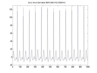
Figure –4 Figure
illustrating the original ECG sample recording
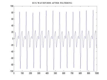
Figure –5 Figure
illustrating the ECG sample recording after applying the filters
Extraction
of the Cepstral Coefficients
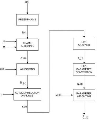
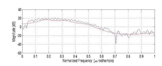
Figure –6 The signal and the LPC log spectra
Solutions Proposed
· HMM with discrete observations
· HMM with continuous observations densities
· HMM with discrete observations used in conjunction with SVM
The choice of HMM to solve this problem is not arbitrary. The data set that we are dealing with is an ECG recording, which consists of a data sequence varying in time. HMM is a dynamic statistical modeling technique that has been previously successfully applied to similar problems in automatic speech recognition applications in the mid-70s. The model’s advantage is that its Markov chain topology preserves the structural characteristics of the data and models the sequence and durations of the waveforms while the model parameters account for the probabilistic nature of the observed data.
For this project, the HMM toolbox by Kevin Murphy was used.
A. HMM with Discrete
Observations
In order to solve the first problem, two HMM models were designed for each of the two classes: subjects with no PAF and subjects with PAF. When implementing HMM, several issues have to be taken into consideration:
· The initial estimates of the model parameters: the state-transition probability distribution A, the observation symbol probability distribution B, and the initial state distribution p.
· The number of states.
· The number of observations.
As far as the first point is concerned, two cases were taken into consideration: uniform initial conditions and random initial conditions. Another approach might be to divide the training data and use a portion of it in order to initial the model parameters, but again there is always the issue of ‘initial estimates of the initial estimates’.
In order to determine the range of states the HMM has, the waveform of a beat was referred to again. As can be seen from the figure below, the heartbeat has been modeled as having 7 states. This is just a proposed model of the beat states but is suggests that 7 states are appropriate for modeling a beat. Accordingly, the number of states was varied between 5 and 8.
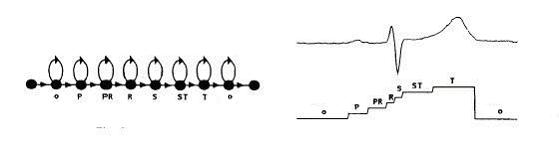
Figure –7 Hidden
Markov Modeling of a Heart Beat
Since the original data was continuous, it had to be discretized. The number of discrete levels was selected to be 20. Furthermore, in order to facilitate the manipulation of the observation probability distribution B, the data was digitized. The figure below shows a block diagram describing the process of digitization. Following that are figures showing the histograms of the PAF and NO PAF training data that helped in the selection of the 20 initial estimates (figures7,8). Hence the data was finally mapped to 1 of 20 symbols. The training was performed using the Baum-Welch algorithm iterated 5 times, and the classification of the test data was performed by calculating the log-likelihood versus each of the two models using the forward procedure.
The second problem was dealt with in a similar manner where two HMM’s were modeled for each of the two classes: subjects with PAF about to experience an attack and subjects with PAF that have not experienced an attack.
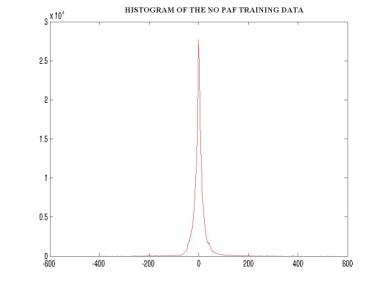
Figure –8
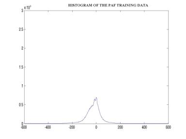
Figure –9
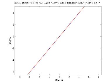
Figure –10
HMM-based classifier applied to cepstral features
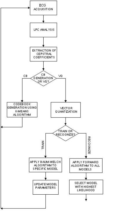
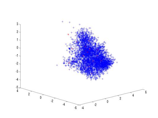
Figure –11 The
cepstral coefficients along with the 32 codebook cepstral vectors (first three
dimensions)
B. HMM with Continuous
Observation Densities
Since HMM can be used to model continuous observation densities and since the waveform morphology would be preserved if the original continuous data set was used, the second attempt to solve the PAF problem used HMM’s with continuous observation densities. The observation densities were modeled as a finite mixture of Gaussian models.
![]() Where N is the
number of states.
Where N is the
number of states.
With this model, two new sets of parameters were added, the mean and variances of the mixture models. The number of means and variances to be estimated was N´M where M is the number of mixture models and N is the number of states. The initial estimates of the means were selected randomly from the training data and k-means was then applied to refine the estimates. The variances were estimated as the sample variances using the training data and the estimated mean.
For the purpose of this project, the number of mixture models, was varied experimentally between 1, 5 and 7.
C. HMM with Discrete
Observations in Conjunction with SVM
The aim of this application is to investigate the combination of a dynamic method, HMM with a discriminative method SVM. In this application, HMM is not used as a classifier rather as an intermediate stage that would provide the appropriate feature vectors for the SVM classifier. One basic concept behind this application is that eventually HMM’s attempt to represent a set of data using a model. The log-likelihood estimate calculated in the recursive forward algorithm measures the closeness of the sequence to a model. However HMM is not a discriminative method in the sense that it can assign the same likelihood to two quite different data sequences. Since HMM is good at modeling at modeling a set of data (given the right criteria), we will use it to do so. The training data for each class is used to train the models. Next all the data sequences are transformed into vectors by representing each into what is know as Fisher Score.
![]()
Which is the derivative of the log-likelihood of the
sequence O with respect to a model parameter ![]() . Thus instead of simply computing the likelihood of a
sequence with respect to an HMM, we are extracting a vector which describes the
extent to which the parameters contribute to generating the specific sequence.
In this case, the parameters with respect to which we will derive are the
observation probabilities. A detailed derivation of the above equation is found
in [2]. For brevity only the final result is included:
. Thus instead of simply computing the likelihood of a
sequence with respect to an HMM, we are extracting a vector which describes the
extent to which the parameters contribute to generating the specific sequence.
In this case, the parameters with respect to which we will derive are the
observation probabilities. A detailed derivation of the above equation is found
in [2]. For brevity only the final result is included:
![]()
![]() can be viewed as the
expected posterior frequency of emitting observation vk which being
in state j. It is calculated using gt(j) which is the probability of being in
state j at time t. The result of this derivation is a N´20 matrix. Where N is the
number of states and 20 is the predetermined number of observation symbols. The
rows are aligned to give a 120-length vector.
can be viewed as the
expected posterior frequency of emitting observation vk which being
in state j. It is calculated using gt(j) which is the probability of being in
state j at time t. The result of this derivation is a N´20 matrix. Where N is the
number of states and 20 is the predetermined number of observation symbols. The
rows are aligned to give a 120-length vector.
Now we turn our attention towards the discriminative technique used. The discriminant function used is:
![]()
The sign of the discriminant function determines whether the test vector belongs to C1 or C2. The next issues to deal with are:
·
How to assign the ![]() ’s.
’s.
·
What is K(O,Oi)
It is important to get good
estimates of the ![]() ’s for the discriminant function to be most likely to have
the right sign. Not only do we want the right sign but we would also like to
have the answer different from zero by a certain margin b. However,
since any margin once achieved can be scaled by scaling the
’s for the discriminant function to be most likely to have
the right sign. Not only do we want the right sign but we would also like to
have the answer different from zero by a certain margin b. However,
since any margin once achieved can be scaled by scaling the ![]() ’s, we can initially simply solve for the coefficients by
imposing an additional constraint of
’s, we can initially simply solve for the coefficients by
imposing an additional constraint of ![]() . Once found, the values can be scaled by the required factor
to get the desired margin. To solve for the
. Once found, the values can be scaled by the required factor
to get the desired margin. To solve for the ![]() ’s we refer to [2] and define a quadratic function for the
coefficients:
’s we refer to [2] and define a quadratic function for the
coefficients:
![]()
![]() ’s are then solved for iteratively:
’s are then solved for iteratively:
Where the sign changes depending on whether the coefficients are C1 or C2.
The function f is such
that f(z)=0 for z![]() 0, f(z)=z for 0
0, f(z)=z for 0![]() z
z![]() 1, and f(z)=1 otherwise.
1, and f(z)=1 otherwise.
For this application, the kernel function used is the Gaussian kernel
![]()
Where D is the distance between the Fisher scores
previously calculated and is given by for the two sequences ![]() and
and ![]() :
:
![]()
Where ![]() is the covariance
matrix of the score vectors in the class of
is the covariance
matrix of the score vectors in the class of ![]() and is approximated
by the identity matrix scaled by a factor s2. s is
set to be the average Euclidean distance between the Fisher scores
corresponding to a given class and the closest Fisher score belonging to a
different class. From the definition of this scaling factor, one can
approximate the distance between a Fisher score from a class C and its nearest
non-member as 1. The method described is referred to in [2] as the SVM-Fisher
method.
and is approximated
by the identity matrix scaled by a factor s2. s is
set to be the average Euclidean distance between the Fisher scores
corresponding to a given class and the closest Fisher score belonging to a
different class. From the definition of this scaling factor, one can
approximate the distance between a Fisher score from a class C and its nearest
non-member as 1. The method described is referred to in [2] as the SVM-Fisher
method.
The following flow chart illustrates and summarizes the different stages used in this application:
Results
·
HMM with continuous observations densities
|
Training Data |
# States |
# Iterations in Baum-Welch |
# Mixtures |
R/U* |
NO PAF |
PAF |
|
5 |
6 |
5 |
7 |
R |
66.66% |
42.2% |
|
25 |
6 |
5 |
7 |
R |
84% |
60% |
|
25 |
7 |
5 |
1 |
U |
80% |
28% |
|
25 |
7 |
5 |
1 |
R |
84% |
32% |
|
25 |
5 |
5 |
1 |
R |
96% |
44% |
|
25 |
5 |
5 |
5 |
R |
96% |
20% |
|
25 |
5 |
5 |
7 |
R |
68% |
80% |
|
Training Data |
# States |
# Iterations in Baum-Welch |
# Mixtures |
R/U* |
PAF episode |
No PAF episode |
|
15 |
6 |
5 |
1 |
R |
90% |
20% |
|
15 |
6 |
5 |
7 |
R |
100% |
0% |
|
15 |
7 |
5 |
1 |
U |
70% |
40% |
|
15 |
7 |
5 |
1 |
R |
80% |
60% |
|
15 |
5 |
5 |
1 |
R |
60% |
70% |
|
15 |
5 |
5 |
5 |
R |
50% |
70% |
|
15 |
5 |
5 |
7 |
R |
50% |
50% |
*R/U refers to whether the initial estimates of the HMM parameters were Random or Uniform.
·
HMM with discrete observations
|
Training Data |
# States |
# Iterations in Baum-Welch |
R/U* |
No PAF |
PAF |
|
5 |
6 |
5 |
R |
22.22% |
82% |
|
25 |
6 |
5 |
R |
76% |
84% |
|
25 |
7 |
5 |
R |
96% |
32% |
|
25 |
7 |
5 |
U |
76% |
72% |
|
25 |
5 |
5 |
R |
76% |
80% |
|
25 |
8 |
5 |
R |
80% |
68% |
|
Training Data |
# States |
# Iterations in Baum-Welch |
R/U* |
PAF episode |
No PAF episode |
|
15 |
6 |
5 |
R |
60% |
30% |
|
15 |
7 |
5 |
R |
40% |
70% |
|
15 |
7 |
5 |
U |
80% |
60% |
|
15 |
5 |
5 |
R |
20% |
100% |
|
15 |
8 |
5 |
R |
80% |
20% |
·
HMM with discrete observations (cepstral
coefficients)
|
Training Data |
# States |
# Iterations in Baum-Welch |
R/U* |
No PAF |
PAF |
|
5 |
5 |
5 |
R |
22.22% |
84% |
|
25 |
5 |
5 |
R |
24% |
84% |
|
25 |
7 |
10 |
R |
36% |
76% |
|
25 |
7 |
10 |
U |
20% |
72% |
|
25 |
6 |
10 |
R |
28% |
72% |
|
25 |
8 |
10 |
R |
16% |
76% |
|
Training Data |
# States |
# Iterations in Baum-Welch |
R/U* |
PAF episode |
No PAF episode |
|
15 |
5 |
5 |
R |
40% |
50% |
|
15 |
7 |
5 |
R |
80% |
0% |
|
15 |
7 |
5 |
U |
60% |
30% |
|
15 |
6 |
5 |
R |
60% |
30% |
|
15 |
8 |
5 |
R |
60% |
40% |
·
HMM with discrete observations used in conjunction
with SVM
|
Training Data |
# States |
# Iterations in Baum-Welch |
R/U* |
No PAF |
PAF |
|
5 |
6 |
5 |
R |
84% |
52% |
|
25 |
6 |
5 |
R |
88% |
88% |
|
25 |
7 |
5 |
R |
96% |
80% |
|
25 |
7 |
5 |
U |
52% |
76% |
|
25 |
5 |
5 |
R |
96% |
76% |
|
25 |
8 |
5 |
R |
84% |
76% |
|
Training Data |
# States |
# Iterations in Baum-Welch |
R/U* |
PAF episode |
No PAF episode |
|
15 |
6 |
5 |
R |
70% |
90% |
|
15 |
7 |
5 |
R |
100% |
90% |
|
15 |
7 |
5 |
U |
40% |
100% |
|
15 |
5 |
5 |
R |
50% |
80% |
|
15 |
8 |
5 |
R |
70% |
70% |
Remarks
· Improvement of results with increase in training data.
· Change of results for random/uniform initialization.
· Change of results with the number of states.
· Change of results with the number of mixture models (HMM with continuous observations densities).
· On average, highest recognition rates for the HMM-SVM method.
References
1. K.-R. Müller, S. Mika, G. Rätsch, K. Tsuda, and B. Schölkopf. An introduction to kernel-based learning algorithms. IEEE Neural Networks, 12(2): 181-201, May 2001.
2. T. Jaakkola, M. Diekhans, D. Haussler. A discriminative framework for detecting remote protein homologies. Journal of Computational Biology, 7:95-114, October 1999.
3. D.A.
Coast, R.M. Stern, G.G. Cano, S.A Briller. An approach to cardiac arrhythmia
analysis using hidden Markov models
Biomedical Engineering, IEEE
Transactions on, 37(9): 826-836, Sept. 1990
4. R.O. Duda, P.E. Hart, D.G. Stork. Pattern Classification 2nd Edition, Wiley Interscience, NY, 2001.
5. L.R. Rabiner, and B. Juang. Fundamentals of Speech Recognition, Prentice-Hall, Englewood Cliffs, NJ, 1993.
6. C.Q. Du, Prediction of Paroxysmal Atrial Fibrillation(PAF) Onset through Measurement of Heart Rate Variability(HRV), Thesis Proposal for the Degree of MEng. in EECS at the Massachusetts Institute of Technology, 2002.