Feature selection,
localisation and first results
The next
step was trying out feature selection on the representations mentioned before,
with two aims in mind:
- Localizing of the features described
by the labels
- Speeding up and enhancing
recognition performance (the traditional aim)
Some first
(and quite acceptable, in some cases) classification performance results also
came out of this process.
What is feature selection?
Feature
selection is the process by which, out of a set of features, we decide to keep
a subset with certain desired properties, mainly in order to speed up and
enhance classification, which will take placed based on the chosen subset. Some
evaluation criterion is chosen, and we are seeking the subset that maximimises
or anyway satisfices it. Such criteria might be:
- “Distances” of probability
distributions of different classes, such as the KL-distance discussed later
- Evaluation of the performance of a
quick-and-dirty classifier on the train set, or on a validation set
Concerning
the choice of subsets to be evaluated, many approaches exist, for example:
- Brute force (combinatorial explosion
is reached fast – 2^n subsets to be tried)
- Brute force with constraints: for
example, all subsets within a certain range of dimensions, or with specific
connectivity / geometric properties etc. In essence, brute force on a specific
set of subsets of the original set.
- SFS/SBS sequential forward /
backward selection, choose/leave k
- SFFS (sequential forward floating
selection), a branch-and-bound type method with reportedly superior results
[1].
- GA’s (genetic algorithms), genomes
encoding feature sets, fitness according to criterion.
In our
case, code for all of the above except GA’s was implemented: unfortunately, the
sffs code was still being debugged while this was written.
Feature selection for
localisation
Here, we
attempt to answer the following question:
For a
specific label (for example, moustache), which pixels (most probably forming
areas) of the image contain the crucial information for recognition? Or, else,
can this thing labelled “moustache” be localised somewhere in the face, based
on the training data?
This has
implications in our case towards justifying the adhoc “cutting out” of a
region, and ultimately in providing better and quicker performance. In other
problems, this might correspond to the determination of where in the sensory
surface (for example, where in the body or in which sensation?) is a labelled
stimulus concentrated. If the labels are words other linguistic primitives, we
are in essence roughly “grounding” the semantics of the label.
The subsets
to be evaluated where chosen by brute force out of the restricted space of all
possible rectangles starting anywhere in the image and having sides belonging
to {4,8,12,16,20,24,28,32}, and three criteria were used: KL distance,
recognition percentage of a simple classifier on the training set, and (just
for a test – as optimising by the test set is definetely cheating) recognition percentage of a simple
classifier on the testing set.
A
symmetrised version (arithmetic mean) of the KL distance was used, divided by
the number of pixels in the subset. Also, the resistor-average KL [2] was tried
out, but for the gaussian case we used later it is equivalent. The
implementation of the KL distance was problematic: early histogram-based
approaches sufferred from zeros, some quick fixes for the 1D case were
successful, but these didn’t generalise well to the multi-D case. Thus, to get
a quick working fix, we estimated means and covariance matrices and used the KL
formula for gaussians [3]. However, there were severe numerical problems in
this case too, due to the often ill-conditioning of the inversion of
covariances.
The simple
classifier consisted of a 1D fisher vector projection (discriminating label
with maximum prior with the union of the rest), followed by gaussian fitting
(based on empirical sigma and mu for each class), empirical priors, and the
associated quadratic decision boundary.
Localisation results
If we
arrange the 23K subsets linearly, here’s a picture of what we get:
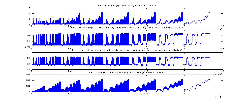
Figure 8: KL, % on train, % on test by subset
index for label 6 (Moustache)
The points to notice are: (other points that exist will become clearer
later)
- Large-scale and small-scale
periodicities due to the looping of rectangle side sizes
- There is certainly a relation
between KL and recognition percentage, of course even more so on the train set.
However, this relation is not always monotonic; there exist pairs of increasing
KL values with decreasing percentages. This was to be expected however, as KL
is related to asymptotic performance, furthermore under other idealisations.
In general, recognition performance of the simple classifier on the
train set was found to be a more reliable predictor of the performance of more
complicated classifiers on the test set than KL, although further
experimentation and quantitative justification is required here.
Even if the original subset areas should be multiples of 16 (4 x 4), as
the subsets were masked by the image mask, all possible areas between one and
the total mask size emerged, with a spiky decreasing histogram. If we now
arrange the subsets by area, we can find the statistics of the criteria as a
function of subset size:
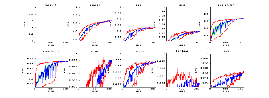
Figure 9: Recognition percentage of simple classifier on train set - statistics as a function of feature set size
(red = min and max, blue = mean,
green = one sigma boundaries), y-axis ABOVE MAX. PRIORS
Points to notice:
- We do get satisfactory separation in
almost all labels – moustache seems best, and race worst
- There are labels for which adequate
information can be found even in small areas of the picture (i.e. are highly
localised); moustache is such a prime example, and also expression. It gets to
90% of its best percentage with a 32-pixel subset, and probably even smaller
(if we allowed all possible rectangle side sizes we would know). I.e.:
'---> LABEL=moustache'
Best KL values [0.50821,4.4972], firstmin@=1, firstmax@=216
But we still get over the
acceptable=4.0475, with an area as small as =211
Best TR perc [0.8673,0.97146], firstmin@=1, firstmax@=152
But we still get over the
acceptable=0.96104, with an area as small as =32
Best TE perc [0.78758,0.93387], firstmin@=1, firstmax@=89
But we still get over the
acceptable=0.91924, with an area as small as =16
- There are other labels where we
continue to get more useful information as the subset size increases, and we
should probably use the whole picture if we can, such as gender. I.e.:
'---> LABEL=gender'
Best KL values [0.12138,0.96421], firstmin@=2,
firstmax@=9
But we still get over the
acceptable=0.86779, with an area as small as =9
Best TR perc [0.61392,0.83926], firstmin@=3, firstmax@=203
But we still get over the
acceptable=0.81292, with an area as small as =132
Best TE perc [0.65731,0.77054], firstmin@=1, firstmax@=130
But we still get over the acceptable=0.75746, with an area as small as =90
- Of course, highly localised labels
have more variance for a fixed size k for small sizes.
Similar results for KL-distances and performance on the testing set ( -
not to be taken into account -) are:
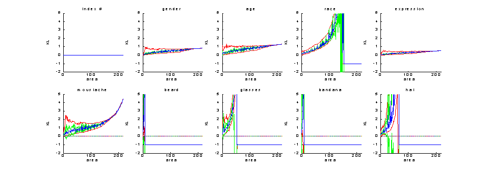
Figure 9: Symmetrised KL distance - statistics as a function of feature set size
(red = min and max, blue = mean,
green = one sigma boundaries), -2 for ill conditioning
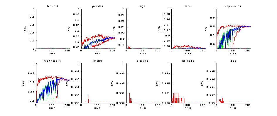
Figure 10: Recognition percentage of simple classifier on test set - statistics as a function of feature set size
(red = min and max, blue = mean,
green = one sigma boundaries), y-axis ABOVE MAX. PRIORS
Here, even if we are not allowed to quote results from feature sets
chosen by performance evaluation on the test set, what will follow becomes
evident by the mean values.
The best feature sets and those at 90% of the performance and minimum
sizes are shown below:
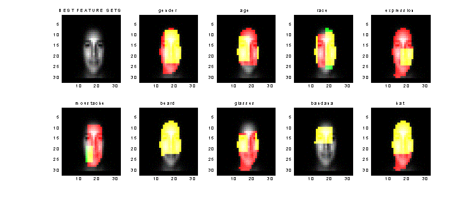
Figure 11: Best feature sets and satisfactory sets (90% of best perf.)
Notice
that indeed the highly localised features require small sets, and also notice
how the inherent symmetry of the human face functions: in many cases, only half
the area is required. We certainly get what we expected for moustache,
expression, glasses, bandana and hat.
If we now plot the number of
times a pixel belongs to a best performing (for size k) feature set over
the number of times it belongs to all sets created, we get the following
informative figures:
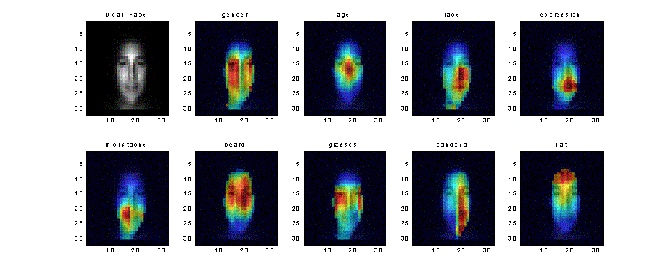
Figure 12: Relative frequency of pixel belonging to best performing sets for size k
(i.e. times pixel belonged to a best performing subset for an area k, k=1:maxk
over times pixel belonged to a feature subset that was evaluated,
where “best performing” is according to rec. perc. on train set by the simple classifier)
Points
worth noting:
-
Localisation is now evident!
We have indeed found out which part of the image is more informative towards
the labels EXPRESSION, MOUSTACHE, GLASSES and HAT.
-
For results with inadequate
rec. performance: the BANDANA result is spurious, due to the fact that two of
the supposedly bandanas are mufflers worn on the neck, and the beard result is
very general due to the suspicious nonlabelling of beards (when a moustache
existed, as pointed out before).
-
It is
interesting that a vertical strip above and below the nose is not informative
towards gender, but this needs further exploration.
-
It would be
worth trying a different set of subsets to start with, or maybe doing some
hierarchical or “zoom in” approach to pixel selection. Definetely in the list
of next steps!
Thus, we have succesfully localised the most important areas for each
label, and thus can justify selecting these. And we have also roughly grounded
words as “moustache” in vision.
Feature
selection on PCA coefficients
PCA
coeffs were calculated for a cut region around the moustache. Preliminary
results show that after selecting the best subset of the form 1:n, selective
deletion of coefficients might incrase performance noticeably (1:18 and then
delete 6, 8..12). Early tests showes increases of more than 3% above the cited
92% for MOUSTACHE, and an ROC area underestimate of . This is definetely worth
further systematic investigation.
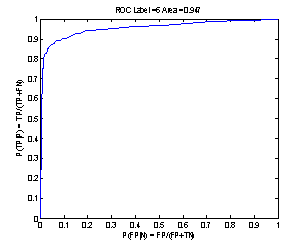
Figure 13: Moustache ROC curve (on test set, by simple classifier) of best subset after feature selection on PCA coeffs
Some
first performance results
Our real results when using the simple classifier with the BEST FEATURE
SETS for the TRAIN set on the test set are:
(i.e. real recognition percentages, with NO involvement of the test set
in tuning)
%(best sets of train on test),
%(small. accept. sets of train on test), %(maxprior), label, %(over maxprior)
gender --->73.9% ,70%
,maxprior=64% , improvement =9.97% ,6.06%
age --->83.8% ,84.4%
,maxprior=86.7% , improvement =-2.86% ,-2.25%
race --->85.1% ,85.3%
,maxprior=85.1% , improvement =-0.0501% ,0.2%
expression --->79.8% ,78.5%
,maxprior=55% , improvement =24.8% ,23.5%
moustache --->91.8% ,91.2%
,maxprior=78.8% , improvement =13.1% ,12.5%
beard --->99.2% ,99.2% ,maxprior=99.5% , improvement =-0.301% ,-0.301%
glasses --->98% ,98.2%
,maxprior=99.6% , improvement =-1.6% ,-1.35%
bandana --->99.5% ,99.5%
,maxprior=99.6% , improvement =-0.0501% ,-0.0501%
hat --->97.7% ,97.6%
,maxprior=99% , improvement =-1.25% ,-1.4%
Thus: (summarising)
Results
for feature selection on pixels and simple classifier:
MOUSTACHE
(~92%), covered 61% of the way from
fixed choice to perfection.
EXPRESSION
(~80%), covered 55% of the way from
fixed choice to perfection.
GENDER
(~74%), covered 28% of the way
from fixed choice to perfection.
Failure
everywhere else, with a near miss in RACE.
Early
evidence of further increase up to 3% (95%) in MOUSTACHE after feature
selection on PCA, in a different cut region
References:
[1]
Jain, A.; Zongker, D. “Feature selection: evaluation, application, and small
sample performance“, Pattern Analysis and Machine Intelligence, IEEE Transactions
on , Volume: 19 Issue: 2 , Feb. 1997, Page(s): 153 -158
[2] Johnson, D.H. and Sinanovic, S. , “Symmetrizing the Kullback-Leibler
Distance”., submitted to Signal Processing Letters, 2002.
[3] Therrien, C. , “Decision, Estimation and Classification”, Wiley,
1989