Supervised Approach to Activity Recognition
This site contains the detailed description of the methodology followed while exploring different supervised machine learning algorithms such as support vector machines, neural nets, decision trees, KNNs, naive Bayesian classifier and hidden markov models to the activity recognition problem.
Is our dataset balanced or unbalanced?
A balanced data is the one for which we have the same number of training examples per class. Otherwise, we have an unbalanced dataset. Thus, our dataset is unbalanced.
|
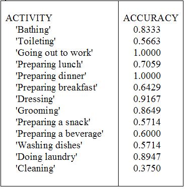
Activities labeled for this experiment
|
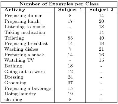
Many of the standard classification algorithms usually assume that training examples are evenly distributed among different classes. However, as indicated in (Japkowicz, 2000), unbalanced data sets often appear in many practical applications.
-
medical diagnosis: 90% healthy, 10% disease
-
eCommerce: 99% don't buy, 1% buy
-
Security: >99.99% of Americans are not terrorists
Studies (Weiss 1995; Kubat, Holte, & Matwin 1998; Fawcett & Provost 1997; Japkowicz & Stephen 2002) show that in many applications, unbalanced class distributions result in poor performances from standard classification algorithms. These classification algorithms generate classifiers that maximize the overall classification accuracy. When dealing with unbalanced data sets, this leads to either trivial classifiers that completely ignore the minority class or classifiers with many small (specific) disjuncts that tend to overfit the training sample.
Some approaches for dealing with unbalanced data include
- Resizing training data (balance it!)
- Adjusting misclassification costs
Undersampling (eliminate examples in majority class)
Oversampling (replicate examples in minority class)
- Recognition-based learning
(learn rules from the minority class examples with or without using the examples of the majority class )
In this work, we run experiments comparing the classification over the unbalanced data vs the balancing using oversampling. The results presented are using unbalanced data since the classification accuracies where not that different and did not feel natural to balance the data given the particular application.
(use cost-sensitive classifiers by setting a high cost to the misclassifications of a minority class)
What classification approach was followed for the sequential data?
1. Sliding windows: converts the sequential supervised learning problem into classical supervised learning problem by constructing a window classifier. The training is done by converting each sequential training example into windows and then applying standard supervised learning algorithms in each window.Works well but do not take advantage of correlation between adjacent windows.
2.Recurrent sliding windows: the predicted value for window in time T is fed as an input to help in the prediction/classification. Common approaches are recurrent neural networks and recurrent and recurrent decision trees. For example in a neural net you can have feedback loops from output nodes to hidden nodes or in the hidden nodes themselves.
3.Hidden Markov models: the premiere approach which includes dependency between 2 consecutive time slices as seen in class.
In this work, we used the sliding window approach (window size=14min spaced each 3min intervals) for all the methods but the HMM for which the Hidden markov model approach was used. The window size is the average duration for all the activitites.
How to avoid False positives?
One of the interesting problems when building recognition systems that will perform in real-time is to reduce the number of false positives. In this application, false positives are not desired since they could cause an undesired interruption in a human computer interaction or a bad judgement of the level of independency while analyzing the activities that a person can carry out everyday.
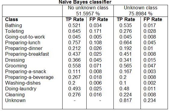
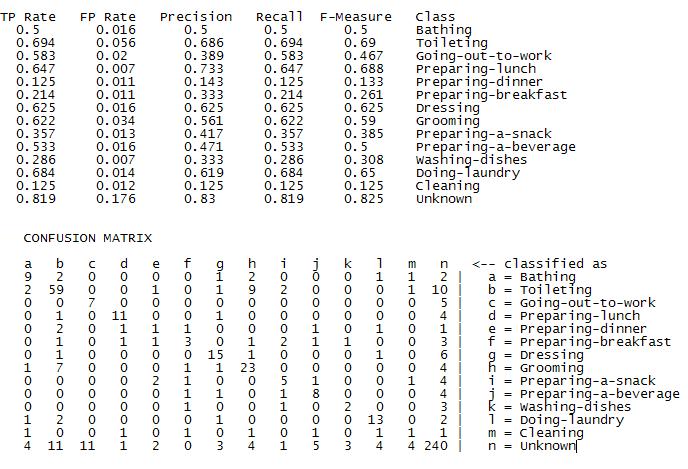
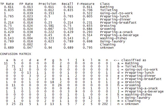
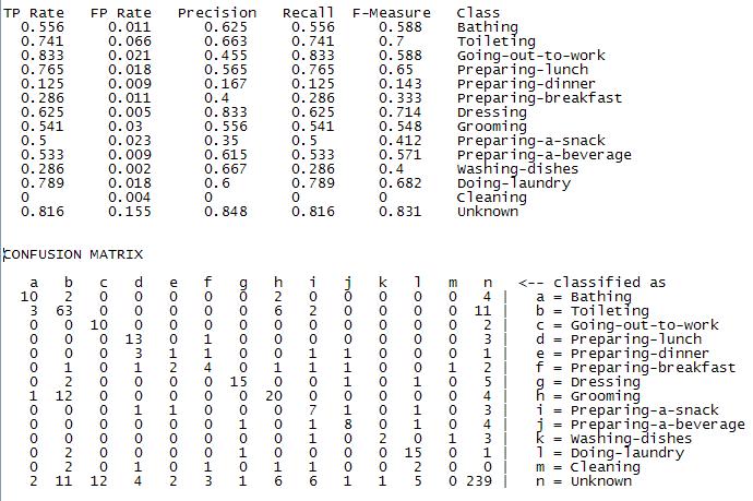
Our approach to try to reduce the false positive rate was to training an new class called 'unknown' from all the unlabeled chunks of data.
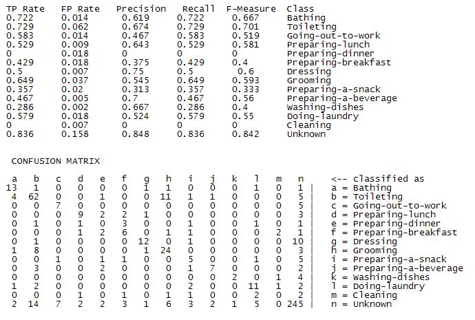
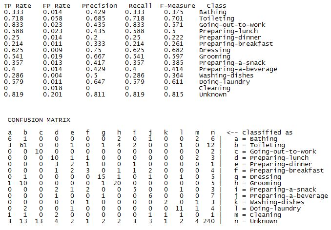
From the following table, we can see that adding the 'unknown' class not only helps in reducing the number of false positives for some of the classes but also helps in the classification performance.
*This results were also verified for the other classifiers
It is worth mentioning that for this particular problem, it is difficult to calculate the number of false positives, since the dataset was labeled using experience sampling and not video. Thus, a considerable number of labels per day are missed. In other words, our algorithms could be correctly classifying the activities but we are missing the labels for those.
Feature Extraction
What features is it possible to extract?
The following features are some of the features that can be calculated from the sensor activations
| Feature | Example of feature vector for one class |
| Count of total sesors activated per activity | [44] |
| Number of ON/OFF transitions | [22] |
| Mean/Variance of sensor activation time | m=[6255] v = [300] in sec |
| Mean/variance of first and last activation time for each sensor | m=[1002] v = [460] in sec |
| Counts of sensor ( IDs) activated | [50 51 66] [0 2 1 ] (could be binary) |
| Count of objects activated | [drawer toilet cabinet] [ 1 2 0 ](could be binary) |
| Count of rooms activated | [kitchen studio bathroom][ 4 9 1 ](could be binary) |
| most likely room in which activity occured | [studio] or [4] |
|
Before fluent for sensors ID (is one sensor activated before another) |
[55_66 2_66 4_33] [1 0 0] (binary) |
| Before fluent for sensor objects(is one sensor activated before another) | [drawer_fridge microwave_cabinet] [1 0] |
What features did we used?
| Feature | Example |
| Objects activated (binary) | [drawer toilet cabinet] [ 1 1 0 ] |
| rooms activated (binary) | [kitchen studio bathroom][ 1 0 1 ] |
| most likely room in which activity occured (nominal) | [studio] or [4] |
Why?
- Discrete attributes could allow fast computation and possible real-time performance
- Could be possible to learn the models of activities for one person and test them on another person provided the sensors are installed in the same locations in each home.
- It is possible to use high level information as prior information to help to reduce the number of training examples required
- Can be possible to apply feature selection and find the most discriminant sensors and reduce system costs
Classifiers Explored
What classifier algorithms were used?
Support Vector Machines
Decision trees
Neural Nets
Naive Bayesian Classifiers
Hidden Markov models
K nearest neighbors
Support Vector Machines
Why did we use support vector machines?
- Maps data in high dimensional space
- Fast prediction (multiplication of inner products)
- sparse solution (decision boundary determined by subset of training points)
What transformations were necessary to the attributes?
SVMs require each instance to be represented as a vector of real numbers. Thus, the nominal attributes were converted to binary valued attributes
example: (Red, green, blue) => (1 0 0), (0 1 0), (0 0 1)
What parameters were used?
We used a SVM with the following parameters
- RBF Kernel
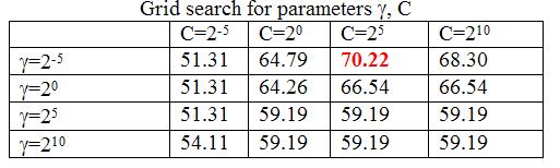
- C = 32, gamma=0.031
How were the parameters selected?
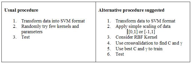
Usually, it is difficult to choose the different parameters of theSVMs. It is a trial and error process that involves the following steps.
 |
 |
Why is the alternative procedure recommended?
- Because RBF kernel handles the non-linearly separable case
- Linear and sigmoid kernels are special cases of the RBF kernel
- Less numerical problems since 0<K
<1
What are the classification results?
| Correctly classified | 70.57% |
| Incorrectly classified | 29.42% |
 |
Comments
RBF kernel seems to map our data well into high dimensional space since classification results are reasonable.
Decision Trees
Why did we use ID3 decision trees?
- No restriction bias, just preference bias
- Fast classification
- Human interpretable results (click for example output)
What transformations were necessary to the attributes?
None, decision trees can handle nominal (discrete) attributes.
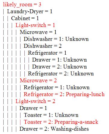
What parameters were used?
No prunning, no other parameters available.
What are the classification results?
| Correctly classified | 68.47% |
| Incorrectly classified | 31.52% |
 |
Comments
Includes feature selection: Comparing the produced decision tree with the ranking of attributes according to the filter method information gain, we can see that the ordering correlates.
Does not capture the majority function well: if we compare the results for the 'unknown' class with the results for the other classifiers, we can see that it has lower accuracy and higher FP rate. DT usually not capture the majority function well since tell would produce large trees
Relatively few attributes determine classification for each class
Neural Networks
Why did we use Feed-forward Multilayer perceptrons?
- Using 2 layers can approximate any arbitrary function provided enough hidden units
- Calculate high level features over the inputs useful for classification
- Input feature vector is high dimensional
- lean the majority function well
What transformations were necessary to the attributes?
Neural nets require each instance to be represented as a vector of real numbers. Thus, the nominal attributes were converted to binary valued attributes. After the conversion, scaling between [-1, 1] was applied. This is suggested for improved performance in neural nets while dealing with nominal attributes
What parameters were used?
We used the following parameters
- One hidden layer
- 250 Training epoch
- learning rate=0.3, no decay
- momentum=0.2
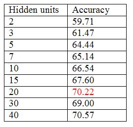
- Number of hidden units=20
- Training using backpropagation (with momentum)
- output codification= distributed encoding (instead of local since output does not fall in linear scale)
How were the parameters selected?
The number of hidden nodes was selected by generating an evidence curve using crossvalidation. Please note that the random initialization values for the nodes weights were kept fixed.
 |
What are the classification results?
| Correctly classified | 70.22% |
| Incorrectly classified | 29.78% |
 |
Comments
Performs well even with the small training data: One possible answer is that it is learning the majority function well for each class and that some complex high level feature extraction is taking place in hidden layer.
Results are difficult to interpret. Model is a collection of weights which are not to meaningful.
Naive Bayesian Classifier
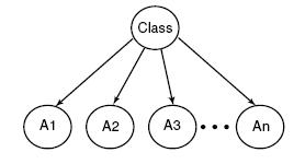 |
Why did we use the naive Bayesian classifier?
- Performs surprisingly well for its simplicity
- Fast training/testing times
- produces probabilistic outputs
- Prior information on the domain can be incorporated
What transformations were necessary to the attributes?
None, works with nominal attributes.
What parameters were used?
We used the following parameters
- Laplacian smoothing for probabilities (adds pseudocounts to avoid zero probs)
- Training by simply counting number of times attributes occur in classes (discrete case)
What are the classification results?
| Correctly classified | 67.77% |
| Incorrectly classified | 32.22% |
 |
Comments
Was interesting to see that it performs well even though its decision boundary is linear
Since NB has so few parameters 2^(n+1) for boolean attributes, it scales well to high dimensions.
Gives the lowes classification accuracy compared to other methods. usually used as a baseline algorithm to compare performances
Hidden Markov Models
Why did we use discrete hidden markov models?
- Takes advantage of time sequence from past state to current state
- Produce probabilistic output
- relatively fast classification time
- Prior information on the domain can be incorporated
What transformations were necessary to the attributes?
Hidden markov models can only use one single discrete attribute. Thus, for this experiment, we decided to use only the number of sensor activated as the discrite attribute. For example, the
What parameters were used?
We used the following parameters
- hidden states=1
- Baum-welch for training
- forward-backwards algorithm for classification
How were the parameters selected?
The number of hidden states was selected by generating an evidence curve using crossvalidation. Please note that the random initialization values for the transition and observation probabilities were kept fixed.
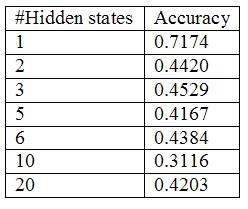 |
What are the classification results?
| Correctly classified | 71.7% |
| Incorrectly classified | 28.3% |
 |
*Accuracy was tested over segmented data
Comments
Only one hidden state does well probably because there is not enough training data.
The hidden markov model works in a similar way to the naive Bayesian classifier
It is performing well compared with the other algorithms although it was tested over segmented data.
K Nearest Neighbor
Why did we use KNN?
- Simple and has proven gives good results, particularly in combination with PCA
- Can be used as a baseline for comparing different algorithms
What transformations were necessary to the attributes?
KNN require each instance to be represented as a vector of real numbers to be able to measure distances. Thus, the nominal attributes were converted to binary valued attributes.
What parameters were used?
We used the following parameters
- Euclidean distance used
- Distance weighting by 1/d
How were the parameters selected?
The number of neighbors was selected by generating an evidence curve using crossvalidation
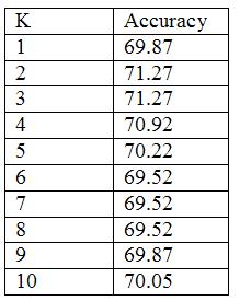 |
What are the classification results?
| Correctly classified | 71.27% |
| Incorrectly classified | 28.72% |
 |
Comments
For its simplicity, it is doing well on the dataset
Finding the two closest examples with most similar sensor activations
Since K is the smoothing factor, small Ks tend to cause overfitting. This might be the case since K=2.
Performing well but requires storing all instances.
Summary of classification results
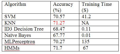 |
Why all algorithms are performing about the same?
Well, we have to remember that our algorithms high depend on the discriminant power of our features. We can have the most powerful classifier in the world but if we have poor features it will perform poorly.
Could we have overfiting in the domain?
The whole process of looking for an algorithm that works well for our data is itself a learning process. While the test data is used for measuring the accuracy of individual algorithms, it is serving as training data for the purpose of selecting an algorithm. It could be that one algorithm did better just because of the variance of the test data.
What algorithms would we finally use for a real-time application?
We would probably use HMMs or Naive Bayesian classifier given their performance, probabilistic output and classification time.
Is this an easy or difficult classification problem?
Well, the dataset is a difficult one. It is unbalanced, is not labeled using video which means that some of the labels are missing and the sensors are noisy. Furthermore, different people label activities differently. Thus, it is a difficult classification problem.
Feature Selection
What features did the Filter method selected?
Using the filter method using information gain were the following:
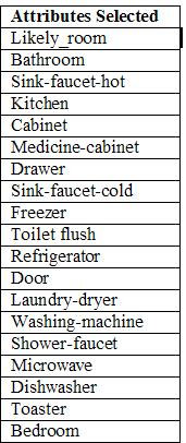 |
Attributes ranked from most important (top) to less important (bottom). Also, only the first 19 attributes are shown
What features does the wrapper method using the naive Bayesian classifier selected?
rom mUsing the wrapper method with the naive Bayesian classifier and best first search we get
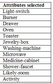 |
Using only the features selected, the classification performance was improved by ~3%
Contact information
Please direct any questions and comments to
Emmanuel Munguia Tapia [emunguiaATmit.edu]
Randy Rockinson [rockinsATmit.edu]