Bayesian Classification
The first classifier I explored was a Bayesian classifier, with
Gaussian distributions. I believed it would work well for
some features, and not well for others. For example, consider
the density feature. I believed that very low densities and very high densities
would lead to bad rhythms. Therefore, there would be
a sweet spot in the middle where all the good patterns were.
The data, however, do not support this hypothesis. Examining the distributions,
there is much overlap between the good and bad classes in track density.
This table describes it:
| Feature | mean (bad) | mean (good) | sigma^2(good) | sigma^2(bad) |
| Clap Density | .6659 | .6603 | .0146 | .0132 |
| Snare Density | .4380 | .4512 | .0150 | .0165 |
| Kick Density | .3563 | .3646 | .0145 | .0153 |
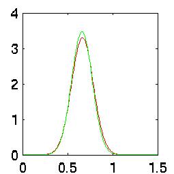
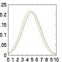
This is even easier to see graphically. The red curve is the bad data, the green curve is the good data.
Recall that the area under each curve is unity. The Bayes error rate is the area underneath
where both curves overlap. In all three of these graphs, you can see that the error rate is
nearly 100%:
 |
| Kick PDF |
 |
| Snare PDF |
 |
| Clap PDF |
Some Better Features
Although the simple density features were not very compatible with
Gaussian classification, one of the nice surprises of this project
was to discover that a few other features were better. For example,
the 8th harmonic, the density of silence (a.k.a. state 0) and the
density of snare drums (state 2) had the highest correct classification
rates when taken independently. The difference is easy to see in their Probability
Density Functions (PDFs):
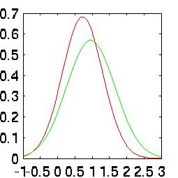 |
| 8th Harmonic |
 |
| Silence Density |
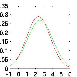 |
| Snare Density |
Taken independently, the correct classification rates for
these three features are:
| Feature | Classifcation Rate |
| 8th Harmonic | 65.89% |
| State 0 Density | 67.44% |
| State 2 Desnity | 62.14% |
A Big Mistake
A big mistake I made was to ignore the curse of dimensionality. Remembering
that with Bayesian classification, additional data can only equal or improve
classification, I hurried to concatenate as many features as possible into
my Bayesian classifier. It was only after I got a miserable classification
rate with all 24 features enabled (54.4%) that I remembered the second half
of the rule: Additional data can only improve Bayes with infinite data sets.
Feature Finding
Then I got curious. I wanted to know the quality of every single feature,
so wrote a matlab script called Feature Find, that classified with Bayes
for every single feature independently (against the validation set). The results were surprising.
The biggest shocker was that many features were classifying
just barely above the priors. (P1 = 59.71%. P2 = 40.42%):
| Classification Rate | Feature # |
| 59.33% | 20 |
| 60.66% | 1 |
| 60.66% | 2 |
| 60.66% | 3 |
| 60.66% | 4 |
| 60.66% | 6 |
| 60.66% | 7 |
| 60.66% | 9 |
| 60.66% | 10 |
| 60.66% | 11 |
| 60.66% | 12 |
| 60.66% | 13 |
| 60.66% | 15 |
| 60.66% | 16 |
| 60.66% | 18 |
| 60.66% | 21 |
| 60.66% | 22 |
| 60.66% | 23 |
| 60.66% | 24 |
| 61.33% | 8 |
| 61.66% | 5 |
| 62.13% | 19 |
| 65.89% | 14 |
| 67.44% | 17 |
Feature Seeking
Given that some features are better than others, I wanted to
know what combinations of features would be best.
Obviously, there are 2^K = 2^24 possible combinations which would
take too long to run, so I wrote a new version of Feature Find
called Feature Seek. This script sequentially classifies, adding
one more feature each time. If the new feature makes the classification
worse, it gets dropped. Otherwise, it gets accumulated.
It is not perfect, but it is interesting and helpful. When I ran
it the first time, I realized it is very biased toward the
first few features. For example, the first feature is always
better than 0, so it always gets picked up and can not be dropped
later. These features might possibly inhibit other useful features.
Therefore, I ran it forwards, from feature 1 to feature 24, then
backwards from 24 to 1. I saw that the best three independent
features did not all survive. Forwards, features 17 and 19 survived,
but 14 did not. Backwards, 14 and 19 survived, but 17 did not.
10 features did not survive either direction.
Because I was rooting
for my favorite features, I decided to try to initialize the
feature enable vector with features 14, 17 and 19, the ones
with the highest independent classification rates. Then, I ran
the forwards and backwards sequential Feature Seek. Interestingly,
these favorite features all remained enabled after sweeping
through forwards and backwards. Clearly, they must be important.
Random Feature Seek
Reconsidering the bias of sequential movement, I made a Random Feature Seek (RFS) script.
RFS picks a feature at random, inverts its enabled/distabled status, classifies,
and keeps the change if it is better. I ran it three times for 200 iterations
each. As the table shows, the selected features were similar to the sequential,
but with no obvious bias toward the first or last features. Also note that this
method produced the highest rate of classifcation for Bayes (71.06%).
Finally, it is interesting to note that in all 7 runs of selecting features,
there were some definite trends. Feature 10, the 4th harmonic, was never selected.
Features 5, 6, 12 and 20, were each picked only once. Features 8, 14, 17 and
19 were the most often picked. What is especially interesting is that
while 8, 14, 17 and 19 were the among the highest independent features, feature
5 was also among the highest independent, but the lowest in combination
with others. Feature 5 represents the evenness, which is a combination of
other features. Therefore, when it is alone, it represents quite a bit of
information. However, in the presence of the other information from which
it is comprised, it has little more to contribute.
(1=Enabled, 0=Disabled)
| Feat. # | Fwd | Bkwd | Init. Fwd | Init. Bwd | Rand1 | Rand2 | Rand3 |
| 1 | 1 | 0 | 1 | 0 | 0 | 1 | 0 |
| 2 | 1 | 0 | 1 | 1 | 1 | 0 | 0 |
| 3 | 1 | 0 | 1 | 0 | 0 | 1 | 0 |
| 4 | 1 | 0 | 0 | 0 | 1 | 0 | 0 |
| 5 | 0 | 0 | 0 | 1 | 0 | 0 | 0 |
| 6 | 1 | 0 | 0 | 0 | 0 | 0 | 0 |
| 7 | 0 | 0 | 0 | 1 | 1 | 1 | 1 |
| 8 | 0 | 1 | 1 | 1 | 1 | 1 | 1 |
| 9 | 0 | 0 | 1 | 1 | 1 | 0 | 1 |
| 10 | 0 | 0 | 0 | 0 | 0 | 0 | 0 |
| 11 | 0 | 1 | 0 | 0 | 1 | 1 | 1 |
| 12 | 0 | 0 | 0 | 0 | 0 | 0 | 1 |
| 13 | 0 | 0 | 1 | 0 | 0 | 0 | 0 |
| 14 | 0 | 1 | 1 | 1 | 1 | 1 | 0 |
| 15 | 0 | 0 | 0 | 1 | 0 | 1 | 0 |
| 16 | 0 | 0 | 0 | 1 | 1 | 1 | 1 |
| 17 | 1 | 0 | 1 | 1 | 1 | 1 | 0 |
| 18 | 0 | 0 | 1 | 0 | 1 | 0 | 0 |
| 19 | 1 | 1 | 1 | 1 | 0 | 1 | 0 |
| 20 | 0 | 0 | 0 | 0 | 1 | 0 | 0 |
| 21 | 0 | 1 | 0 | 1 | 1 | 0 | 1 |
| 22 | 0 | 1 | 0 | 0 | 1 | 0 | 1 |
| 23 | 0 | 1 | 0 | 1 | 0 | 0 | 1 |
| 24 | 0 | 1 | 0 | 1 | 0 | 0 | 0 |
| rate: | 66.48% | 67.73% | 70.39% | 69.08% | 67.76% |
69.74% | 71.06 % |
Results
The correct classification rate for the group of features
that tested highest against the validation data is 52.20%.
--->General Linear Discriminant
Index