General Linear Discriminant
I wanted to try using a GLD next, because it is a fairly simple algorithm.
It executes very rapidly, so I could do plenty of experimentation with
different combinations of features. Based on what I had seen of the
distributions of data earlier, though, I suspected it might not work well.
This is because GLD builds boundaries from polynomials. I suspected
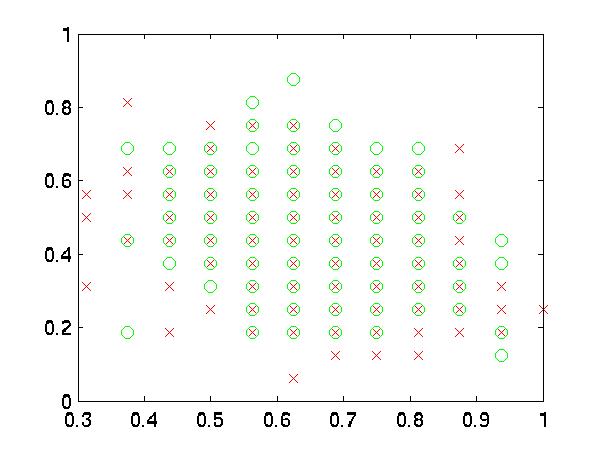
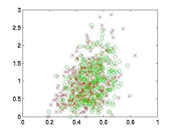
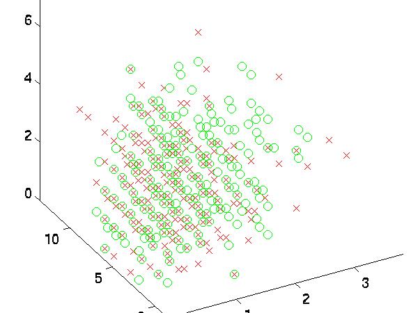
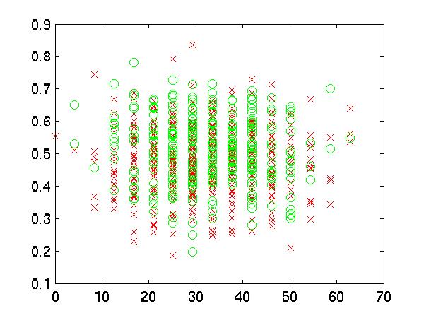
the boundaries of my data were very complex. To test this I graphed some features
against each other. As you can see, the two datasets "good" and "bad"
are almost hopelessly intertwined for most features.
 |
| 1 vs. 2 |
 |
| 5 vs. 8 |
 |
| 17 vs. 10 |
 |
| 14 vs. 17 vs. 19 |
The Good Features
Similar to what I had done with Bayes, I used random feature-seeking
to find the best features. They seemed to be 5, 6, 10, 12 and 17.
| Feat. # | Rand1 | Rand2 | Rand3 |
| 1 | 0 | 0 | 0 |
| 2 | 0 | 0 | 0 |
| 3 | 1 | 0 | 0 |
| 4 | 1 | 0 | 0 |
| 5 | 1 | 0 | 1 |
| 6 | 1 | 0 | 1 |
| 7 | 0 | 0 | 0 |
| 8 | 1 | 0 | 0 |
| 9 | 0 | 0 | 0 |
| 10 | 0 | 1 | 1 |
| 11 | 0 | 0 | 0 |
| 12 | 1 | 1 | 0 |
| 13 | 0 | 0 | 1 |
| 14 | 1 | 0 | 0 |
| 15 | 1 | 0 | 1 |
| 16 | 0 | 0 | 0 |
| 17 | 1 | 1 | 1 |
| 18 | 0 | 0 | 0 |
| 19 | 0 | 1 | 0 |
| 20 | 0 | 0 | 0 |
| 21 | 1 | 0 | 0 |
| 22 | 1 | 0 | 0 |
| 23 | 1 | 0 | 0 |
| 24 | 0 | 0 | 1 |
| rate: | 65.13% | 65.79% | 66.48% |
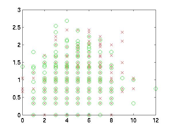
Then, I graphed these features against each other. It is pretty clear
that there is no low order polynomial boundary to separate them. But
scientists have to be very, very sure. For example,
some graphs have the same color at both fringes that might be useful
in classifcation:
|
| 17 vs. 10 |
 |
| 6 vs. 5 |
 |
| 12 vs. 17 |
Results
Therefore, I experimented with values 2 and 4 for K. K=2 improved
classification somewhat, probably picking up those fringes with its parabola shape.
K=4 performed miserably at 50/50!
| Polynomial Order (K) | Validation Classification Rate | Correct Classification Rate |
| 1 | 57.2% | 55.9% |
| 2 | 58.1% | 56.6% |
| 4 | 52.3% | 50.0% |
--->Fischer Linear Discriminant
Index