Fischer Linear Discriminant
The FLD technique is primarily a way to reduce dimensions. It does this
such that the distributions of the reduced data are maximally separate for Gaussian
criteria. In other words, the new means of the two reduced sets are as far apart as possible,
while maintaining the new variances as small as possible. Reducing to a single dimension for classification,
which I did here, is probably the simplest application of Fischer Discriminants, although it is
possible to reduce to other dimensions as well.
I was pleasantly surprised by this technique. I underestimated it completely. I
thought it would perform only slightly better than Bayesian classification. This is because
following the dimension reduction, a conventional Bayes classification takes place. True, the FLD technique
improves the separation, but I did not anticipate it would be so good. In fact, this turned out
to be the most accurate classifier.
As usual, I began by surveying the features against the validation data one at a time. I was impressed by how many
of them (22 out of 24) were higher than the priors:
| rate | Feat # |
| 60.4167 | 7 |
| 60.4167 | 21 |
| 62.5000 | 14 |
| 64.5833 | 5 |
| 64.5833 | 17 |
| 66.6667 | 1 |
| 66.6667 | 2 |
| 66.6667 | 3 |
| 66.6667 | 4 |
| 66.6667 | 6 |
| 66.6667 | 8 |
| 66.6667 | 9 |
| 66.6667 | 10 |
| 66.6667 | 11 |
| 66.6667 | 12 |
| 66.6667 | 13 |
| 66.6667 | 15 |
| 66.6667 | 16 |
| 66.6667 | 18 |
| 66.6667 | 20 |
| 66.6667 | 22 |
| 66.6667 | 23 |
| 66.6667 | 24 |
| 68.7500 | 19 |
Improved Feature Separation
FLD improves separation of otherwise lousy features.
For example,
remember the track density features examined in detail in the Bayesian classification section?
FLD improved them significantly:
| Feature | Bayes Class. Rate w/o FLD | Bayes w/ FLD |
| Kick Density | 60.66% | 66.66% |
| Snare Density | 60.66% | 66.66% |
| Clap Density | 60.66% | 66.66% |
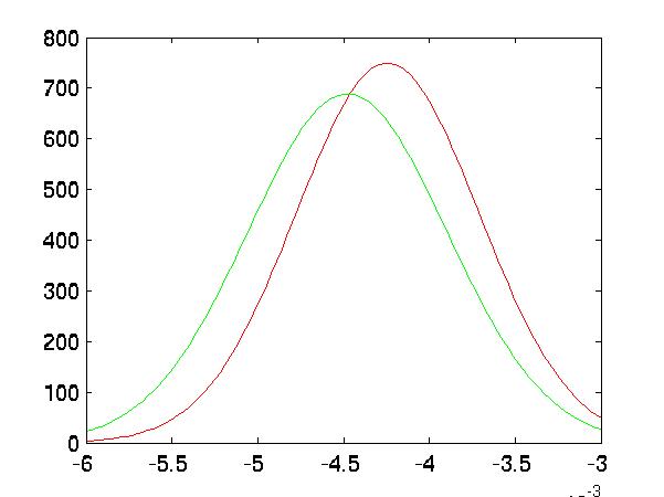
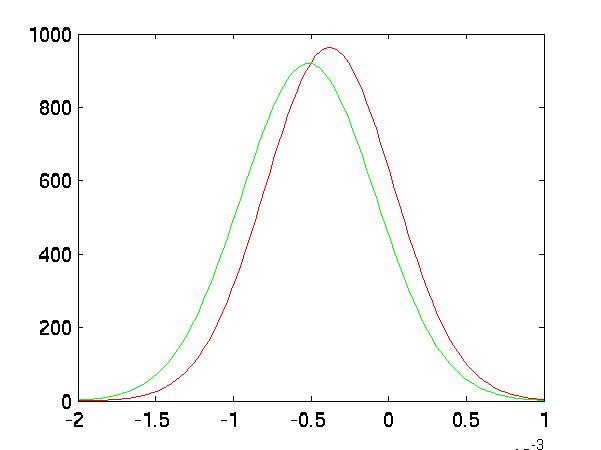
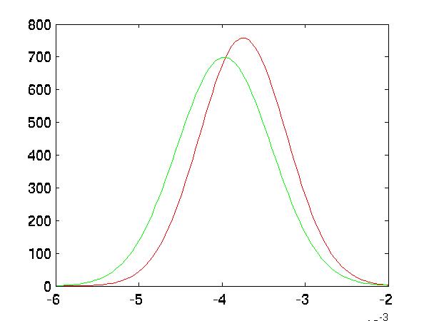
One can also see this in the graphs of their distributions. The FLD transformed the
datasets into more separable ones. This is most clear in features 2 and 3, although not
necessarily in feature 1. Also notice the vertical axis. The pre-FLD distributions
had maximum heights at around 4. The FLD transform significantly narrowed the
distributions, lowering the variances radically:
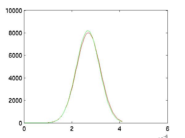 |
| Feature 1 after FLD |
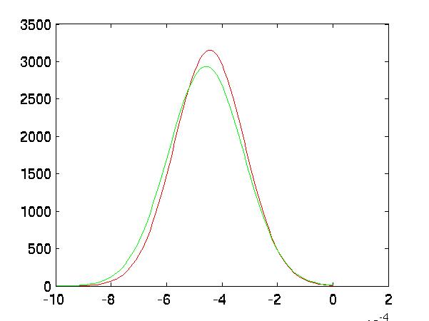 |
| Feature 2 after FLD |
 |
| Feature 3 after FLD |
Next, I selected groups of potentially useful features using forward, backward and random
processes and tested them:
| feature | Fwd | Bkwd | Rand 1 | Rand 2 | Rand 3 |
| 1 | 1 | 0 | 1 | 0 | 0 |
| 2 | 1 | 0 | 1 | 1 | 1 |
| 3 | 1 | 0 | 1 | 0 | 1 |
| 4 | 0 | 0 | 0 | 0 | 1 |
| 5 | 1 | 0 | 1 | 0 | 1 |
| 6 | 1 | 0 | 0 | 1 | 0 |
| 7 | 1 | 0 | 0 | 1 | 1 |
| 8 | 1 | 1 | 1 | 1 | 1 |
| 9 | 0 | 0 | 1 | 0 | 0 |
| 10 | 0 | 1 | 0 | 1 | 0 |
| 11 | 1 | 0 | 1 | 0 | 0 |
| 12 | 1 | 1 | 1 | 0 | 1 |
| 13 | 1 | 0 | 0 | 0 | 1 |
| 14 | 0 | 0 | 0 | 0 | 0 |
| 15 | 0 | 0 | 0 | 1 | 0 |
| 16 | 1 | 1 | 1 | 0 | 1 |
| 17 | 0 | 0 | 1 | 1 | 0 |
| 18 | 1 | 1 | 0 | 1 | 1 |
| 19 | 0 | 0 | 0 | 1 | 0 |
| 20 | 1 | 1 | 1 | 0 | 0 |
| 21 | 0 | 1 | 1 | 1 | 0 |
| 22 | 0 | 1 | 1 | 1 | 0 |
| 23 | 1 | 1 | 0 | 1 | 0 |
| 24 | 0 | 1 | 1 | 0 | 1 |
| Validation Rate | 75.00% | 66.66% | 64.5833% | 72.9167% | 77.08% |
| Testing Rate | 60.3% | 58.1% | 61.0% | 56.6% | 61.03% |
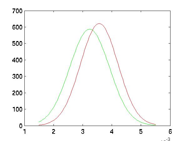
Improved Separation
In the following five graphs, I graph the distributions of the classes after
FLD reduction:
 |
| Forward Selected Distributions |
 |
| Backward Selected Distributions |
 |
| Random #1 Selected Distributions |
 |
| Random #2 Selected Distributions |
 |
| Random #3 Selected Distributions |
Cheating
Just out of curiousity, I executed the random feature seeking
script against the testing data in order to find the theoretical
maximum possible classification. It reached a maximum value of
65.44%. This result can not be counted toward actual classification,
it is just a reference number that suggests how much better the
classification might be able to get with more data.
Results
The correct classification rate for the group of features
that tested highest against the validation data is 61.03%.
--->k Nearest Neighbor
Index