The Effect of Feature Selection on Classification of High Dimensional Data

MAS.622J

Fall 2006

Meredith Gerber

1. Problem

The Differential Mobility Spectrometer (DMS) is a promising technology for differentiating biochemical samples outside of a lab setting, but it is still emerging and analysis techniques are not yet standardized.

The DMS is a micromachined device that separates compounds based on the difference in their mobilities at high and low electric fields (Miller, Eiceman et al. 2000). (See Figure 1.)

Figure 1. Mode of DMS detection. Chemical separation in the DMS is achieved due to an alternating electric

field that is transverse to the direction of carrier gas flow. Changes in the DC compensation voltage allow

different compounds to pass through to the detector according to differences in mobilities between the high

and low fields. Image from (Krylova, Krylov et al. 2003).

The DMS has been used in laboratory settings for differentiating biologically-relevant chemical samples (Shnayderman, Mansfield et al. 2005), demonstrating that different bacteria, and even different growth phases of the same bacteria have distinct chemical characteristics that the DMS can detect.

DMS technology has even been applied in non-laboratory settings demonstrating its potential as a compact, reagent-less, fiieldable sensor technology (Snyder, Dworzanski et al. 2004).

Analysis of this data is particularly challenging for two reasons:

1) The high dimensional nature of the data

2) The difficult link between identifiable data features and specific chemical compounds

What I show here are potential directions and points of consideration for pattern recognition problems involving high-dimensional data, with an eye towards selecting features with clear chemical relevance from high-dimensional data.

2. Data

The entire data set consists of 100 samples in each of three different classes corresponding to the material sampled: Bovine Serum Albumin (BSA), Ovalbumin (OVA), and water. Data were split into a training/testing subset (90%) and a sequestered validation subset (10%) randomly. In the training/testing subset of the data there were 85 BSA samples, 92 OVA samples, and 93 water samples. The training/testing set will be used to optimize parameters and feature sets, and the validation set will be used to validate parameters and selected features.

Each file has 98,000 dimensions corresponding to unique combinations of three different variables: scan number, compensation voltage (Vc), and polarity. When the positive and negative spectra are placed next to each other (even though they are recorded at the same time), each data file can be thought of as a matrix, the entries of which vary in two dimensions, uniquely, according to the chemical composition of the sample. (See Figure 2.)

B

A

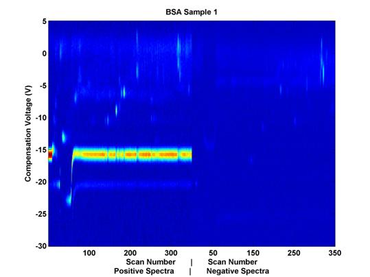
Figure 2. Example Data Sample. Compensation voltage is on the vertical axis and scan number (elution time)

is on the horizontal axis. The positive and negative spectra are placed next to each other horizontally,

for visualization purposes, but as their scan numbers indicate, the data were collected simultaneously.

(A) indicates the Reactant Ion Potential (RIP), and (B) indicates some chemical features which may be of

interest from a classification perspective as well.

The color represents sensor output values; the noticeable horizontal line (A) at compensation voltage -15 is the Reactant Ion Potential (RIP). It is mostly an artifact of the carrier gas with which the sample travels through the system. It is not hypothesized to yield relevant chemical data. The activity of interest seems to occur at compensation voltages of -14 and higher. These data have already been trimmed for relevance in the time domain, but an additional trimming here in the voltage domain could be beneficial in that it will help to remove from consideration nearly half of the remaining features.

All of the data have been pre-processed prior to this analysis. They have been trimmed in the time domain in addition to having been background-adjusted so that the baseline value is common across all samples.

The biggest pattern recognition problem here is the curse of dimensionality. The dimensionality of each sample is about 98,000 and there are 100 samples per class. The challenge is to create a system/classifier that given an input can determine the underlying class of that input--ie, diseased or not diseased, with accuracy, given limited space/memory and limited time. This is a problem that is common in different biology applications (such as DMS, mass spectrometry, and microarray analysis).

3. Approaches

Feature selection has been performed on the training/testing data set so far with two approaches:

1. Two-class Fisher Linear Discriminant

2. PCA

In all cases, 50 features were selected from the data, and classification was performed with a range of numbers of features, between 1 and 50, to demonstrate trends in classification as the number of features used is changed. Additionally, features were selected at a range of radial distances from previously selected features (measured in scan-Vc space pixels). This was done to decrease the degree of correlation between selected features. The specific numbers of features and radial distances were:

Number of features used: [1 3 5 10 20 30 50]

Radial distances used: [1 2 3 5 8 10]

Classification has been performed with SVM (polynomial kernel) and K-Nearest Neighbors (K-NN) with a range of values for K:

Values for K: [1 3 7 11]

3.1 Fisher Discriminant, Two-Class (FLD)

For each pixel, the Fisher Linear Discriminant was calculated as indicated in Equation 1 (Duda, Hart et al. 2001). Pixels were considered as potential features and the features with the highest discriminant values were retained.

(1)

Where μ represents the mean of the pixel values across all samples and σ² is the variance of the values. The maximum values were between 1 and 1.5 and the range of values can be seen in Figure 3.

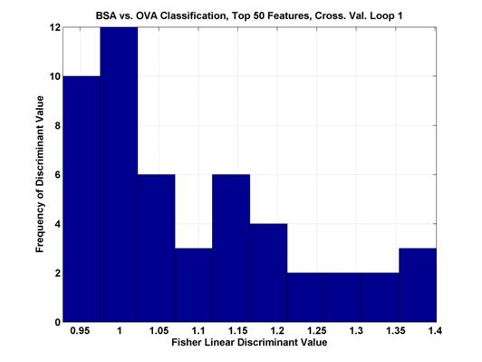
Figure 3. Histogram of the top 50 Fisher Linear Discriminant values. In the first cross-validation loop of the two

class comparison between BSA and OVA. The higher the discriminant value, the more separable the two classes.

The features with the highest Fisher Linear Discriminants are sent to the classifier for classification. However, in many cases, these features are not independent. Each pixel is a potential feature, but as can be seen in Figure 2, chemical features encompass a range of scans and compensation voltages. Potential features which are near to each other (in scan number and compensation voltage) are more likely to be correlated (in their information content).

3.2 Principal Component Analysis (PCA)

A dimension reduction approach was implemented using PCA. Rather than selecting specific pre-existing features, PCA extracts features from the original data, making linear combinations of potential features resulting in a feature set with lower dimensionality than the original feature set. In this case, however, features with clear chemical identity were desired, so a traditional PCA approach was modified to create a feature selector that would yield specific (scan number, Vc) points.

The eigen-decompisition step of PCA is space/memory intensive. In order to make this feasible, the dimensionality of the data had to be further reduced prior to feature selection. First, a subset of the data was selected in scan-Vc space (see Figure 4). Then, further reduction was achieved by down-sampling this space until fewer than 5,000 dimensions remained (out of an original 98,000.

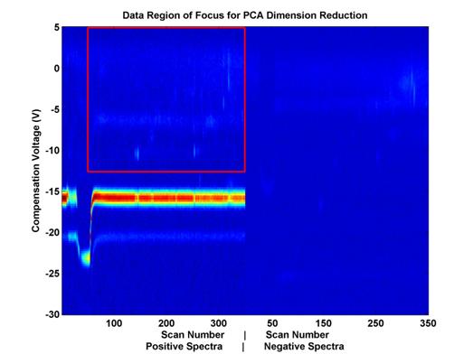
Figure 4. Feature space covered by PCA analysis. This space includes about 21,000 out of 98,000

potential features from the data displayed. This number of potential features had to be further reduced

in order to perform PCA because of space and memory constraints. To further reduce the potential

number of features, this space was evenly sampled.

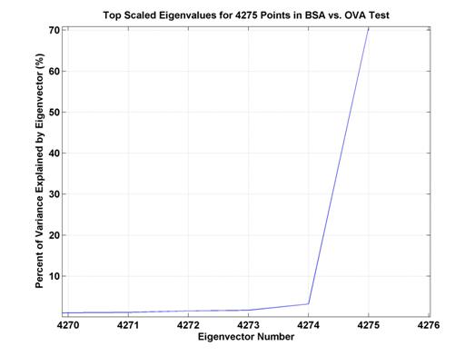
Figure 5. Percent of variance explained by top several eigenvectors. The top eigenvector explains

a bit over 70% of the variance whereas the second eigenvector only accounts for slightly more than 3%

of the variance.

E

D

C

B

A

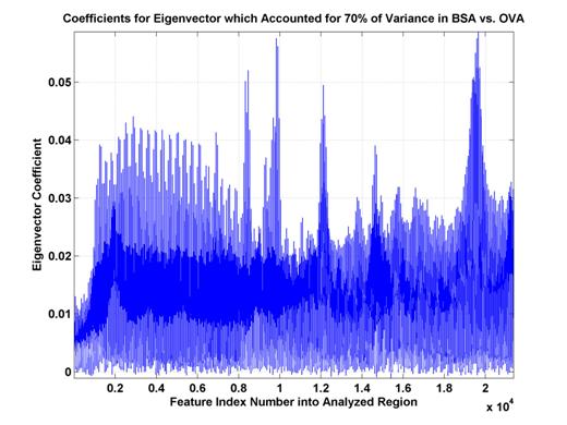
Figure 6. Eigenvector coefficients for top eigenvector. These coefficients explain 70% of the

variance of the distribution of (training and test) data. Some sets of high coefficient feature

indices are consecutive (A,B,C,D) while another has a sinusoidal nature (E). This likely indicates

features which are either more oriented along the scan- or Vc-axes.

4. Results

4.1 FLD

Figure 7. Classification Performance for Water vs. BSA (SVM) FLD feature selection. Note that classification

improves as features are added, until about 30 features. Also, note that classification at this point is generally

better with a higher radius rule, likely because selected features are not as correlated.

Figure 8. Classification Performance for Water vs. BSA (K-NN, K=7) FLD feature selection. Note that

performance and trends are generally to similar to those with SVM (see Figure 7). Classification improves as features

are added, until about 30 features. Also, note that classification at this point is generally better with a higher radius

rule, likely because selected features are not as correlated.

Summary of FLD classification results
At r=3, 30 features

Comparison	SVM	K-NN, K=7
H2O vs. BSA	93%	94%
H2O vs. OVA	96%	95%
BSA vs. OVA	83%	88%

Table 1. Classification Performance Summary for FLD feature selection. These are results of classification with 4-fold

cross-validation on the training/testing data set. The K=7 K-NN classifier was chosen as a point of comparison for

the SVM results.

4.2 PCA

Figure 9. Classification Performance for Water vs. BSA (K-NN, K=7), PCA feature selection. Compare to results

with FLD feature selection (Figure 8). Trends are similar, though classification accuracy is not as good, in comparison.

Summary of PCA classification results
At r=3, 30 features

Comparison	SVM	K-NN, K=7
H2O vs. BSA	88%	90%
H2O vs. OVA	84%	88%
BSA vs. OVA	85%	86%

Table 2. Classification Performance Summary for PCA feature selection. These are results of classification with 4-fold

cross-validation on the training/testing data set. The K=7 K-NN classifier was chosen as a point of comparison for

the SVM results.

6. References

Duda, R. O., P. E. Hart, et al. (2001). Pattern Classification, John Wiley & Sons.

Krylova, N. S., E. Krylov, et al. (2003). "Effect of Moisture on the Field Dependence of Mobility for Gas-Phase Ions of Organophosphorus Compounds at Atmospheric Pressure with Field Asymmetric Ion Mobility Spectrometry." Journal of Physical Chemistry A 107: 3648-3654.

Miller, R. A., G. A. Eiceman, et al. (2000). "A novel micromachined high-field asymmetric waveform-ion mobility spectrometer." Sensors and Actuators B 67: 300-306.

Shnayderman, M., B. Mansfield, et al. (2005). "Species-specific bacteria identification using differential mobility spectrometry and bioinformatics pattern recognition." Anal Chem 77(18): 5930-7.

Snyder, A. P., J. P. Dworzanski, et al. (2004). "Correlation of mass spectrometry identified bacterial biomarkers from a fielded pyrolysis-gas chromatography- ion mobility spectrometry biodetector with the microbiological gram stain classification scheme." Analytical Chemistry 76: 6492-6499.