Classification
This section covers the actual pattern recognition phase of the project. We describe the algorithms that we use for dimensionality reduction (pca), as well as for classifying the data (linear regression, k-NN, Parzen k-NN).
(In the second part Aaron will eventually describe how we realized that our data set most likely isn't linear and that algorithms such as SVM (Support Vector Machines) and Neural nets.)
We considered a number of different algorithms for classifying the MySpace data set. Since it is generally hard to know in advance which algorithm suits your data set best, we made the decision to try several approaches. In the first stage we our initial data set consisted of 20 features (see: background section). We started off by making the rather risky assumption that our data is linear and thus decided to try out two linear algorithms: linear regression and k-nearest neighbor.
Linear regression using matrix pseudo inverse
In statistics, linear regression simply means a regression method of modeling the expected value of a variable, given the values of some other variable or variables. In our case, we have to be able to handle several simultaneous linear equations. This can be realized by using matrix notations and operations. We create matrix Y, where each row consists of the values for a data point in the data set. Our training data set consists of 400 data points, each having 20 feature values. Thus, our Y array will have the dimensions (600*20). Further, we have our true rating values for social and promotion for each data point - a (600*2) matrix. let us call this matrix b. Now, we have the equation:
Y * a = b
Our goal is to find the weight/transformation vector that satisfies this equation. Since we know the dimensions of Y and b, we know that a has the dimensions (20*2). Since Y isn't square we cannot simply use the inverse to get a. However, we can solve the equation by calculating the pseudo inverse of Y:
a = (Yt*Y)^-1*Yt*b = pinv(Y)*b
We then used a on the test data set to see how well the linear regression algorithm performs. The following graphs illustrate the results:
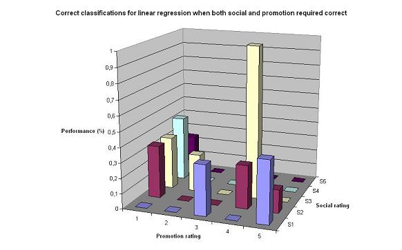
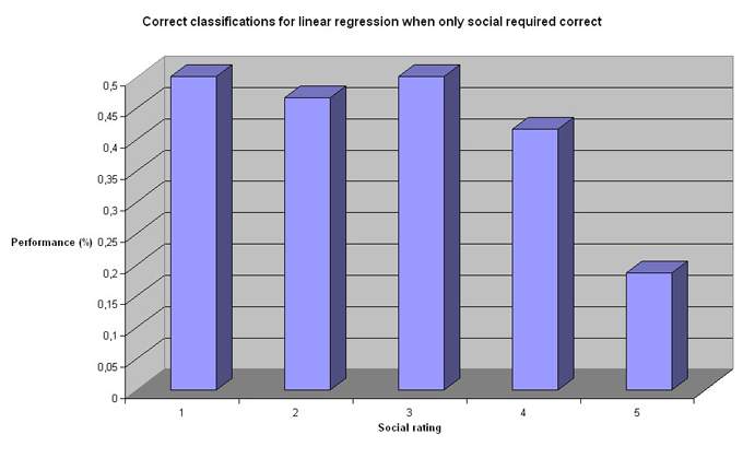

The linear regression classifiers performance is not remarkable, but still quite acceptable. Particularly considering that random is 1/5 = 12.5%, a performance around 50% is good. As expected, the performance is worse when both rating have to be correct. The question is, though. How exact does the classifier have to be? Indeed, filters are more about finding a sufficient threshold, rather than exact values. In our case, we defined spam as high promotion, low social (promotion higher than 1). Therefore, we decided to test the performance for different thresholds for promotion (1,2,3,4) and social <= 2, as well as separate thresholds for social and promotion. The result are presented in the charts below:
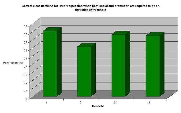
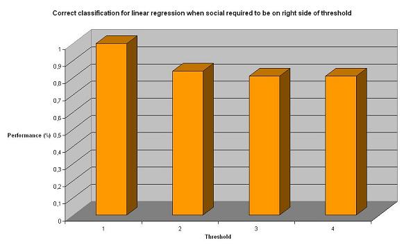
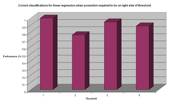
As expected, relaxing the criteria makes the classifier perform significantly better. We now got results over 70-80%, which we consider as really good results. However, we still wanted to test other approaches to see if they could perform even better.
k-NN and Parzen k-NN
k-nearest neighbor (kNN) is a fairly easy algorithm. The basic idea is to classify a specific data point based on the classification of the k nearest neighbors in the (multidimensional) feature space. Thus, k is the number of neighbors that are taken into account. The best choice of k depends on the data and can be found for example by using cross-validation. Euclidean distance is often used as a metric for the distance between the data points. Another version of k-NN is to use a window (e.g. Parzen) rather than a specific number k to determine which data points are to be taken into account. In this case, a window refers to a radius, an area or a sphere. More specifically, all data points that are within a certain range from the current data point are considered. This approach avoids the problem with deviant and distant data points that may distort the results. The question is, ones you have distinguished the group of data points that are to determine the class of the current data point, how do you calculate the class. Is it simply the average of all the values? There are several possibilities. We decided to use voting. Voting means that rather than calculating an average (which in our case would generate values that don't exist in our discrete scale) we choose based on majority. Thus, the result set 1,2,2,4,5 would give 2. The result set 1,2,3,3,2,5 would generate the average of 2 and 3, since we have a tie.
While testing the performance of k-NN, we decided to use leave-one-out cross-validation to find the best number k, as well as the radius for the Parzen window. In the case of kNN, we got k = 1 as the ultimate k for all tested criteria. For k-nn Parzen window we got a similar maximum for social correct, promotion correct, and social+promotion correct. The graphs below illustrate the evidence curves of the different training sessions.
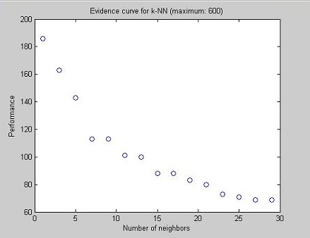
The performance has been calculated for each odd value for k, between 1 and 29. We get a maximum value for k = 1, which indicates that the clusters are weak (non-existing). Since taking more than one neighbor into account makes the classifier more confused, the data seems to be overlapping a lot.
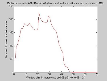
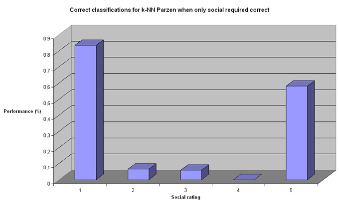
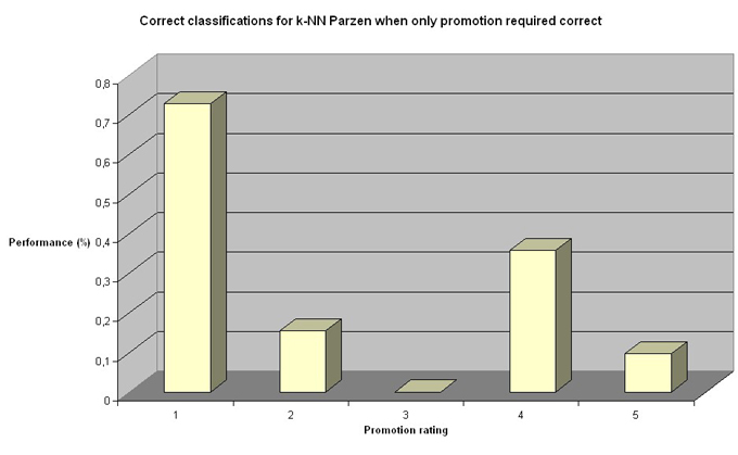
When we use a Parzen window rather than k to determine the result, we get maximum for r = 21*0.05 = 1.05. The distances for the different testing data points vary between 0 and 3.1046. Thus, 1.05 is slightly less than the average distance. The following figures show the result of the testing:
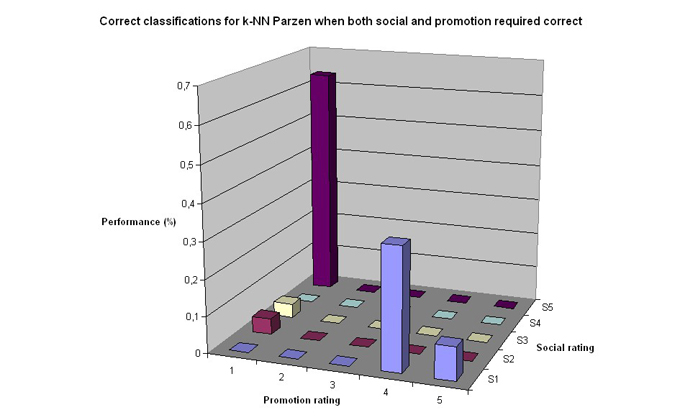
Quite clearly k-NN Parzen performs worse than linear regression. k-NN Parzen performs well in one case: social 1 and promotion 5. This is the data set that is over representative in the data set (see: chart in section Data analysis). The two charts actually look very much the same. It is possible that k-NN Parzen performs worse because it is more sensitive to the uneven data distribution.
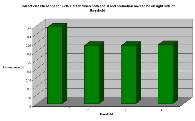
k-NN performs worse than linear regression in all categories. Even when we apply thresholds, the results are ~50%, rather than 80% as seen in the case of linear regression.
Principal Component Analysis (PCA)
So far, we have taken all 20 features into account. The question is if that is necessary? In most cases there are features that are more significant for discrimination than others. Therefore, we decided to test Principal Component Analysis (PCA) to reduce the number of dimensions. The decision to use PCA can and should be questioned, since PCA is known to be better for optimizing representaion, rather than for classification. Despite this, we decided to go with PCA first. It should be pointed out that we have intentions of trying FLD in the near future (Aaron). For PCA, we tried several different numbers of dimensions (top 5, top 10, and top 15 principal components). Here below, we show the results for linear regression and regular k-NN, and k-NN with 5, 10, and 15 features:
In the tables, the values are all performance rate, whereas the scale 1:5 is the rating. In other words, we can see that for rating = 1 for "Linear promo pca 15" has the value 0.96. This means that Linear regression with pca reduction to 15 features, when only the promotion rating is required to be correct, classified 95% of the data points that have promotion rating = 1 correctly. In the same way, for rating = 3, "Linear threshold social pca 5" has the value 0.72. This means that Linear regression with pca reduction to 5 features, when only social has to be on the right side of the threshold 3, classified 72% of the data points correctly.
| 1 | 2 | 3 | 4 | 5 | |
| Linear social pca 15 | 0,61 | 0,27 | 0,21 | 0,08 | 0,02 |
| Linear promo pca 15 | 0,96 | 0,15 | 0,13 | 0,00 | 0,02 |
| Linearthreshold social pca 15 | 1,00 | 0,71 | 0,72 | 0,71 | |
| Linear threshold promotion pca 15 | 1,00 | 0,72 | 0,66 | 0,64 | |
| Linear social pca 10 | 0,74 | 0,29 | 0,26 | 0,04 | 0,00 |
| Linear promo pca 10 | 0,89 | 0,23 | 0,25 | 0,00 | 0,03 |
| Lienar threshold social pca 10 | 1,00 | 0,73 | 0,71 | 0,69 | |
| Linear threshold promotion pca 10 | 1,00 | 0,77 | 0,73 | 0,67 | |
| Linear social pca 5 | 0,52 | 0,27 | 0,35 | 0,33 | 0,05 |
| Linear promo pca 5 | 0,43 | 0,23 | 0,38 | 0,29 | 0,19 |
| Linear threshold social pca 5 | 1,00 | 0,70 | 0,72 | 0,74 | |
| Linear threshold promotion pca 5 | 1,00 | 0,68 | 0,76 | 0,78 |
The chart shows that the PCA dimensionality reduction does not improve the results. As a matter of fact, the threshold classifier performs less well when more dimensions have been reduced.
| 1 | 2 | 3 | 4 | 5 | |
| k-NN social pca 15 | 0,39 | 0,51 | 0,09 | 0,21 | 0,51 |
| k-NN promo pca 15 | 0,75 | 0,08 | 0,00 | 0,14 | 0,47 |
| k-NN threshold social pca 15 | 0,70 | 0,62 | 0,69 | 0,73 | |
| k-NN threshold promotion pca 15 | 0,68 | 0,73 | 0,75 | 0,72 | |
| k-NN social pca 10 | 0,46 | 0,49 | 0,09 | 0,21 | 0,47 |
| k-NN promo pca 10 | 0,80 | 0,00 | 0,00 | 0,29 | 0,40 |
| k-NN threshold social pca 10 | 0,72 | 0,62 | 0,69 | 0,73 | |
| k-NN threshold promotion pca 10 | 0,72 | 0,75 | 0,78 | 0,71 | |
| k-NN social pca 5 | 0,48 | 0,29 | 0,24 | 0,33 | 0,37 |
| k-NN promo pca 5 | 0,61 | 0,08 | 0,00 | 0,07 | 0,50 |
| k-NN threshold social pca 5 | 0,76 | 0,66 | 0,67 | 0,75 | |
| k-NN threshold promotion pca 5 | 0,64 | 0,69 | 0,69 | 0,70 |
k-NN seems to pretty good at detecting values to the right in the chart, i.e. high social or high promotion. It performs worse than linear regression though.
| 1 | 2 | 3 | 4 | 5 | |
| k-NN Parzen social pca 15 | 0,91 | 0,00 | 0,00 | 0,04 | 0,07 |
| k-NN Parzen promo pca 15 | 0,73 | 0,08 | 0,00 | 0,29 | 0,10 |
| k-NN Parzen threshold social pca 15 | 0,33 | 0,49 | 0,69 | 0,78 | |
| k-NN Parzen threshold promotion pca 15 | 0,52 | 0,58 | 0,6 | 0,68 | |
| k-NN Parzen social pca 10 | 0,89 | 0,00 | 0,00 | 0,04 | 0,09 |
| k-NN Parzen promo pca 10 | 0,71 | 0,08 | 0,00 | 0,29 | 0,10 |
| k-NN Parzen threshold social pca 10 | 0,33 | 0,49 | 0,70 | 0,78 | |
| k-NN Parzen threshold promotion pca 10 | 0,52 | 0,57 | 0,59 | 0,68 | |
| k-NN Parzen social pca 5 | 1,00 | 0,07 | 0,00 | 0,00 | 0,00 |
| k-NN Parzen promo pca 5 | 0,91 | 0,00 | 0,00 | 0,00 | 0,00 |
| k-NN Parzen threshold social pca 5 | 0,29 | 0,50 | 0,67 | 0,79 | |
| k-NN Parzen threshold promotion pca 5 | 0,48 | 0,54 | 0,58 | 0,69 |
It seams like, in general, linear regression is better at classifying data points that are on the left-hand side of the chart, i.e. low-promotion or low-social data points. Linear regression gets several 100% correct ones in this area. None of the three approaches are overwhelmingly good. A combination of linear regression and k-NN Parzen would however cover almost the whole spectrum of data points, from low social and/or low promotion to high social and/or high promotion. Now, if we compare the PCA-results with the results and charts above (without PCA), we see an improvement for low social or promotion (left-hand side of chart) for linear regression. Other values (right-hand side) do however not improve by reducing the number of dimensions with PCA. In the case of k-NN and k-NN Parzen, no significant improvements can be seen.
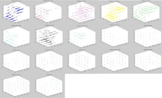
Now, the question is: If PCA can't improve our results, can we, just by plotting the data "get to know" the features better. In other words, can we just by looking at figures of the data distribution distinguish which features are significant or not? Let's look at the data distribution again (see: section Background.
Click on the image to see a high resolution vesion. There is one chart per feature. All charts have the same axes: x: values (0:1), y: social rating, z: promotion rating.