Black Box Classification
Restatement of Problem
Using two feature sets of 11 and 96 dimensions, discuss and quantify the performance of a classifier or multiple classifiers to answer the following questions:
- Given a set of features describing all Prosper listings, can you classify whether or not a listing will become a loan?
- Given a set of features describing all Prosper loans, can you classify whether or not a loan will default?
Motivation
A group of classifiers that perform well for the two problems listed above are of interest to Prosper.com lenders Prosper. Peer to peer lending sites and traditional lending institutions differ in the simple fact that lenders, in most cases, do not have the same sophisticated tools or expert knowledge to properly evaluate risk. Is it possible to build several classifiers that a) filter listing data (question 1 rephrased) and b) filter those users who are least likely to default (question 2 rephrased) so that a lender can maximize portfolio performance. Additionally, these tools are of interest to Prosper. Defaulted and repurchased loans cost Prosper time and money. When a loan defaults, a third party collection agency is brought in to collect any remaining assets. While these tools may not perform a level comparable to those of a lending institution, it will be demonstrated that they perform better than randomly guessing. It is unverified how these classifiers perform compared to a trained expert.
Additionally, if a peer to peer lending company were to implement some smart filters based on these classification results, the peer to peer lending company would reduce the number of loans that defaulted. Lenders would feel more comfortable using a system where they felt they had an investment edge. Overall, the peer to peer company’s track record of loan performance could be greatly improved.
Classification Goals
- Of the classifiers considered, find one (or several) that best fit(s) the datasets in questions 1 and 2 above. In seeking a classifier that fit the datasets well, classifiers were considered in order of increasing complexity.
- For a particular classifier, compare the classification error when using an 11 dimension and 96 dimension feature vector. Ultimately, we want to answer whether or not our intuition of using 11 simple features yields satisfactory performance, versus of the complexity of a feature search to find a near optimal combination of 96 features.
Sampling the Population
First, 4 feature vectors were created for the two specific questions (one of 11 vectors “FS11” and one of 96 vectors “FS96”). It is worth noting that in creating a dataset to answer the loan \ no loan question, the number of available data points for either class were quite disparate. Therefore, to obtain a representative sample stratified sampling was used. This ensures that ratio of the sample priors was kept proportional to the ratio of the entire population. The underrepresented class, in this case, is c1, the number of listings that become a loan. For the 11 vector feature set, the ratio of the priors (prevalence) of c1, is 16.8%. In the 96 vector feature set, the ratio of the priors is 8.5%. In sampling the population for the second set of feature vectors, the ratio of c1/c2 was roughly equal and both classes was sampled randomly.
The sampling size for both feature sets was set at 2000, 5000, and 10,000 samples. For example, an FS96 stratified sample used in a loan no loan classification would contain 850 samples of c1 and 9150 samples of c2.
Classifier Performance
source code for this analysis (matlab)
In summary, the performance of four different types of classification methods is given below. For each classifier, its performance with regards to the two questions above is given. In addition, the performance of classifier with regards to the two feature sets is given.
Method
As mentioned earlier, an empirical study of 4 types of classifiers was conducted.
-
Linear Discriminant, computed using pseudoinverse.
-
PCA+LDA, project dataset onto n principal components and perform a classification using the pseudoinverse.
-
SVM - Linear, 1 norm (SMO) soft margin (slack).
-
Neural Networks: Feedforward. Training method: conjugate gradient descent with one hidden layer.
The method in 1) is simple and straightforward, it was useful in evaluating a baseline performance using all features. The goal behind classification using the principal components of the dataset is that we can reduce the dimensionality of the feature vector yet still account for large of amount in the first few principal components. However, in the case of the 96 dimensional feature vector, multiple principal components must be used in the classifier. Additionally, more computationally expensive techniques such as support vector machines and neural networks are also considered. The goal behind SVM is that by increasing the dimensionality of feature space lower classification error is possible. The SMO training algorithm reduces computational overhead and conserves memory, allowing a larger sample set to be tested. The motivation for using a feedforward neural network is that by adding a hidden layer and finding an optimal number of hidden nodes, we can create arbitrarily complex decision boundaries. The non linear mapping of the neural network is perfect for performing classification on a feature vector with many dimensions.
Performance Tables
These are the methods used:
| SVM(All) | All columns of the feature vector are included in the analysis |
| SVM Top 10 | The top 10 features returned from the floating feature search algorithm were included in the analysis |
| PCA+LDA (10 PC): | A projection of the dataset onto the first 10 principal components was included in the analysis |
| NN ALL (N Hidden): | All dimensions of data included. Number of hidden nodes in the neural network (used primarily to check against over fitting). |
| LDA N: | The number of features considered in calculating the simple linear discriminant. This is primarily intended to compare the performance of the floating feature search to that of 11 feature vector. |
| FS96 E, FS10 E | The error in classification. |
| #FS96, #FS10 | The number of samples used in classification |
| Ratio FS96, FS10 | The ratio of the class to the sample population, or in the case of stratified sampling, to the original population. |
| Tr/(Val)/Te | The percent of sample data used as training, validation, and test. |
| CV FS96, CV FS11 | The type of cross validation used, if any. |
| Null | This particular case was not tested. |
Performance Table of Question 1: “Given a set of features describing all Prosper listings, can you classify whether or not a listing will become a loan?”
The first table “Listing Conversion A” contains the results for using stratified sampling; the second table “Listing Conversion B” contains the results for using random sampling of equal priors.
|
Listing Conversion 1. A |
|
|
|
|
|
|
|
|
|
|
Method |
FS96 E |
FS10 E |
#FS96 |
#FS10 |
Ratio FS96 |
Ratio FS10 |
Tr/(Val)/Te |
CV FS96 |
CV FS11 |
|
SVM (All) |
0.085 |
0.157 |
2000 |
2000 |
0.085 |
0.168 |
70/30 |
None |
None |
|
SVM TOP 10 |
0.098 |
null |
2000 |
2000 |
0.085 |
0.168 |
70/30 |
None |
None |
|
PCA+LDA (10 P.C.) |
0.259 |
0.223 |
5000 |
5000 |
0.085 |
0.168 |
70/30 |
10 Fold CV |
10 Fold CV |
|
NN ALL (20 Hidden) |
0.085 |
0.143 |
2000 |
2000 |
0.085 |
0.168 |
75/15/10 |
N/A |
N/A |
|
NN ALL (10 Hidden) |
0.085 |
0.141 |
2000 |
2000 |
0.085 |
0.168 |
75/15/10 |
N/A |
N/A |
|
NN ALL (5 Hidden) |
0.085 |
0.145 |
2000 |
2000 |
0.085 |
0.168 |
75/15/10 |
N/A |
N/A |
|
LDA 30 |
0.085 |
null |
10000 |
null |
0.085 |
null |
70/30 |
None |
null |
|
LDA 10 |
0.085 |
0.141 |
10000 |
10000 |
0.085 |
0.168 |
70/30 |
None |
10 Fold CV |
|
LDA 5 |
0.085 |
null |
10000 |
null |
0.085 |
null |
70/30 |
None |
null |
|
|
|
|
|
|
|
|
|
|
|
|
Listing Conversion 1.B |
|
|
|
|
|
|
|
|
|
|
Method |
FS96 E |
FS10 E |
#FS96 |
#FS11 |
Ratio FS96 |
Ratio FS11 |
Tr/(Val)/Te |
CV FS96 |
CV FS11 |
|
SVM (All) |
0.190 |
0.270 |
2000 |
2000 |
0.500 |
0.500 |
70/30 |
None |
None |
|
SVM TOP 10 |
0.210 |
null |
2000 |
2000 |
0.500 |
0.500 |
70/30 |
None |
None |
|
PCA+LDA (10 P.C.) |
0.197 |
0.250 |
2000 |
2000 |
0.500 |
0.500 |
70/30 |
10 Fold CV |
10 Fold CV |
|
NN ALL (20 Hidden) |
0.152 |
0.264 |
2000 |
2000 |
0.500 |
0.500 |
75/15/10 |
N/A |
N/A |
|
NN ALL (10 Hidden) |
0.156 |
0.271 |
2000 |
2000 |
0.500 |
0.500 |
75/15/10 |
N/A |
N/A |
|
NN ALL (5 Hidden) |
0.164 |
0.273 |
2000 |
2000 |
0.500 |
0.500 |
75/15/10 |
N/A |
N/A |
|
LDA 30 |
0.273 |
null |
1000 |
null |
0.500 |
null |
70/30 |
None |
null |
|
LDA 11 |
0.257 |
0.240 |
1000 |
2000 |
0.500 |
0.500 |
70/30 |
None |
10 Fold CV |
|
LDA 5 |
0.248 |
null |
1000 |
null |
null |
null |
70/30 |
None |
null |
Table 1. Loan / No Loan Classifier Performance Table
Performance Table of Question 2: “Given a set of features describing all Prosper loans, can you classify whether or not a loan will default?”
|
Default / No Default |
|
|
|
|
|
|
|
|
|
|
Method |
FS96 E |
FS10 E |
#FS96 |
#FS10 |
Ratio FS96 |
Ratio FS10 |
Tr/(Val)/Te |
CV FS96 |
CV FS11 |
|
SVM (All) |
0.190 |
0.270 |
2000 |
2000 |
0.500 |
0.500 |
70/30 |
None |
None |
|
SVM TOP 10 |
0.210 |
null |
2000 |
2000 |
0.500 |
0.500 |
70/30 |
None |
None |
|
PCA+LDA (10 P.C.) |
0.197 |
0.250 |
2000 |
2000 |
0.500 |
0.500 |
70/30 |
10 Fold CV |
10 Fold CV |
|
NN ALL (20 Hidden) |
0.152 |
0.264 |
2000 |
2000 |
0.500 |
0.500 |
75/15/10 |
N/A |
N/A |
|
NN ALL (10 Hidden) |
0.156 |
0.271 |
2000 |
2000 |
0.500 |
0.500 |
75/15/10 |
N/A |
N/A |
|
NN ALL (5 Hidden) |
0.164 |
0.273 |
2000 |
2000 |
0.500 |
0.500 |
75/15/10 |
N/A |
N/A |
|
LDA 30 |
0.273 |
null |
1000 |
null |
0.500 |
null |
70/30 |
None |
null |
|
LDA 11 |
0.257 |
0.240 |
1000 |
2000 |
0.500 |
0.500 |
70/30 |
None |
10 Fold CV |
|
LDA 5 |
0.248 |
null |
1000 |
null |
null |
null |
70/30 |
None |
null |
Table 2. Default / No Default Classifier Performance Table
Discussion of Performance of Loan / No Loan Classifiers (Question 1)
Looking at the error rates of the stratified sample set and the equal prior sample set, you immediately conclude that for all classifiers, with the exception of PCA+LDA, that the stratified sample has a high classification accuracy. In almost every classifier trained and tested with stratified data, the error rate equals the ratio of the prior probability of c1, the number of listings that became a loan. We can thus conclude that while the classifier is correctly classifying all TN samples (c2) we are misclassifying c1. Thus our number of FN equals our classification error. To fix this, we need to alter the classifier slightly, to take into account the cost of misclassifying class 1. This would improve performance.
When comparing data from the Listing Conversion 1.B table, you can see that the FS10 error table exhibits less variance than that of the FS96 error table, suggesting that given 10 features, or a lower dimensional representation of the two patterns, the algorithms perform to a similar degree of accuracy, but this may just be a coincidence of the features selected. We must be careful in making comparisons between the two error tables. While it appears that the FS96 error table is lower than that of the FS10 table, we can only conclude, definitively, that the higher dimensional methods SVM and more degrees of freedom are better suited for this particular 96 dimension feature set.
It is also important to remember that in Listing Conversion Table 1.B are sampled from equal priors and we may have represented class 1 poorly (changed the mean and covariance of the feature vector). In this case, any classification results or conclusions made from this table are somewhat inconclusive. Instead, efforts should be made to find the correct costs in order to penalize incorrect decisions using the stratified data set. Perhaps with more experience, this insight would have been applied up front, and not after the fact.
Discussion of Performance of No Default / Default (Question 2)
Judging classifier performance for this particular pattern of data is straightforward. The variance of the FS10 error column is low, indicating that both both simple and complex techniques classified this particular feature vector to roughly the same degree of accuracy. In this case, one might want to explore how a larger sample set might effect the performance of the classifiers, or similar to the above discussion, test the sample size for goodness of fit.
Inspecting the error table for the FS96 feature set it is clear that the neural network classifier fits the dataset quite well and results in the lowest overall error.
Lessons Learned & Future Improvements
For analyzing these particular patterns, neural networks performed remarkably well. It is not quite surprising given their ability to map complex decision boundaries. We tested several numbers of hidden states, and although DHS recommends n/10 * (training size) number of hidden nodes (where n is the number of data points), we found that the error was relatively stable around 5-20 nodes. With concerns of over fitting, we judged that 20 nodes was sufficient. The fact that these classifiers performed quite well is indicative of the data, simple decision boundaries may not work well given the tendency of feature vectors to cluster in complex manners (review our floating feature selection slides).
Most importantly, the feature selection algorithm should also encompass the classification stage. In more detail, the feature selection routine should be designed in a way such that cross validation is performed at each iteration of inclusion or rejection of a feature. That way, when the algorithm completes, you have your correct answer. Additionally, a smaller sample size should be selected and it should be one that is thoroughly tested against the original population to ensure it’s a correct representation. That way, the algorithm can actually complete running.
However, other less computationally tests exist for finding a good number of features to use in a classifier. That was the idea behind representing the 96 feature vectors in a lower dimensional space. Alternatively, in comparison with other research fields, it appears that 96 dimensions is not an inconceivably large feature vector. From an analytical standpoint, reduction of dimensions is quite tractable, if the error rates are acceptable, represents a perfectly good solution.
One interesting problem that remains unanswered is reducing the remaining 8.5% error resulting from FN classifications in Table A.1 At this point, we have identified how and why that error is there. Certainly stratified sampling is the first correct step, but perhaps there are better methods rather than simply adding more hidden nodes to the neural classifier. One idea revolves around the feature selection routine minimizing the number of FN cases. Again, this raises the issue determining the correct costs for misclassification.
Conclusion
We have demonstrated the performance of several classifiers fit to two different datasets for solving two types classification problems related to the Prosper Data. We have concluded that classifying whether or not a user may or may net get a loan is 8.5% yet this value is not a satisfactory conclusion. Therefore, a classifier built using equally sampled priors is discussed. In this case, the estimated error is 14%. We concluded that a neural network classification of the FS96 dataset was a satisfactory solution and calculated a 15% error rate. Finally, we discuss classification improvements and suggest ideas to improve the classification accuracy of the loans/listings dataset.
Appendix A
Performance Figures
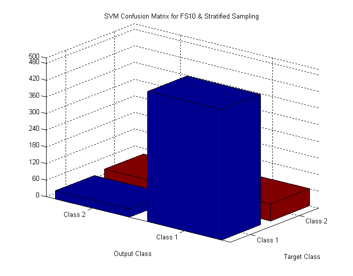
Confusion Matrix for Stratified Sampling Set (FS10)
Typical Confusion matrix for classifier performance in table 1.A
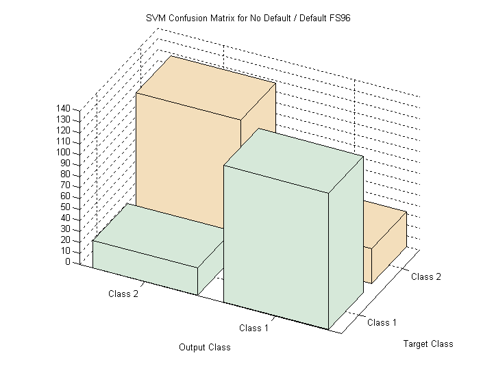
Confusion Matrix for Equal Priors Sampling Set (FS96)
Typical Confusion matrix for classifier performance in table 2
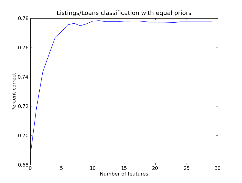
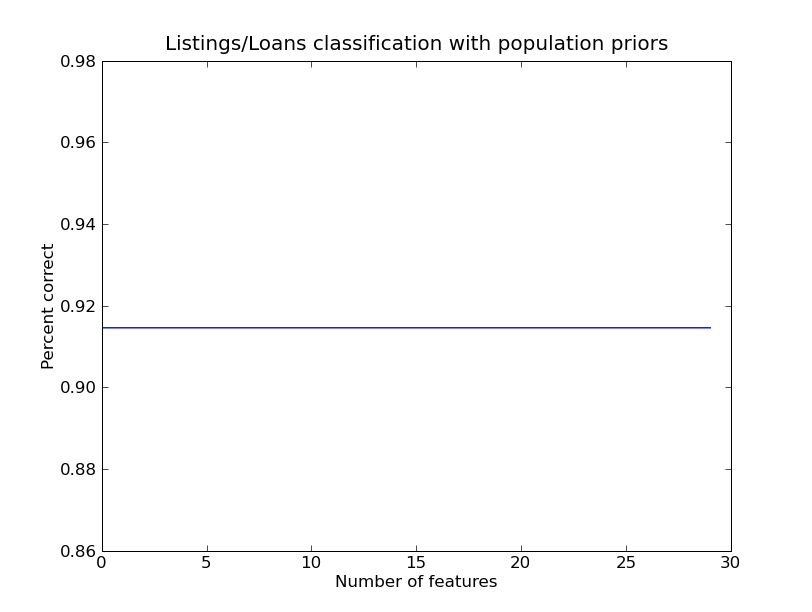
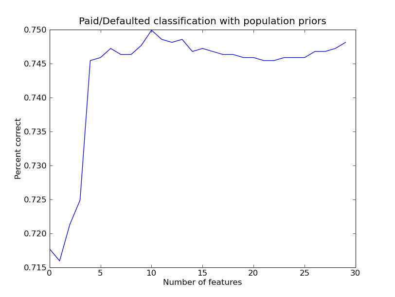
LD Performance Figures for FS96
Testing performance for FS96, note Listings / Loans with Population Priors
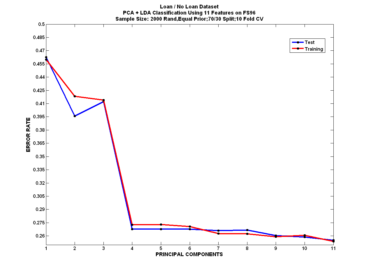
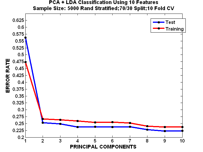
PCA+LD Performance Figures for FS10 For Loan Conversion Table1.A
Training and Testing Curves
PCA+LD Performance Figures for FS96 For Loan Conversion Table1.B
Training and Testing Curves