Decision Trees
Decision tree analysis was used to answer our two original questions about loan conversion and default rate, as well as to suggest ways in which a borrower, a lender, and Prosper.com might each optimize his/its strategy in using the marketplace.
From the borrower’s perspective, some relevant questions include:
- Will I get a loan?
- How much should I request?
- What maximum interest rate should I set?
The lender might ask an inverse set of questions:
- If I fund this loan, can I expect to make a profit?
- At what interest rates am I most likely to optimize overall performance?
- Which profile features best predict a borrower who won’t default?
In turn, Prosper.com is concerned with its own profit maximization:
- How can we increase loan conversion?
- Where can we intervene to prevent default? Should we create a “default insurance”?
- If loans are securitized, can we safely assign different risk ‘classes’ with some robustness?
For a company considering Prosper’s business model (for example, for purchase or VC valuation):
- Is Prosper’s peer-to-peer model viable?
- Do quantifiable features robustly predict performance, or is there too much noise?
Methods
We experimented with several sets of features drawn from the “Original 11” (minus Bid Count) in our decision tree analysis:
- Amount Requested
- Interest Rate
- Credit Score
- Debt to Income Ratio
- Is member part of a group?
- Does listing have image?
- Current Delinquencies
- Delinquencies in Past 7 Years
- Open Credit Lines
- Income
To find the best set of trees to answer each of our questions, we iterated our testing over different thresholds for the division at each node. We aimed to minimize the Gini impurity and find the optimum among different levels of samples per node split:
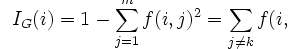
Here, f(i,j) is the probability at a given node that a sample i belongs to a category j. As Ig(i) goes to zero, the samples are all part of a single target category j. Another method used to determine decision tree splits is to minimize information entropy; with the prosper data, we adhere to the Gini impurity.
The node split threshold is the minimum number of observations that a node must have in order to be spit. We experimented with thresholds ranging from 2 to 6400 samples.
We then tested model robustness of various sample-node split combinations by reserving 10% of samples as testing data. We performed testing over 10 iterations of holdout data to consider variation between trees created for a given feature and node-split pair.
Finally, we considered the effect of accounting for prior probabilities. This was a more relevant question in the case of loan vs. no loan, where the data used showed a 13% - 87% split between loans and non-converted listings (we needed to discard some non-loan samples because of missing data, thus the ratio was different from the 10% - 90% split observed in the Prosper dataset as a whole). The use of prior probabilities was less important in the case of default vs. paid: here, the ratio was already quite close to 50% - 50%.
Our point of entry was the classregtree algorithm in MATLAB’s Statistics Toolbox. We made various modifications and additions to the code in order to:
- better visualize the tree output
- take into account (and compare the effect of accounting for) prior probabilities
- create a holdout sample of testing data and iterate over several sets of training/testing data to test model sensitivity
- iterate over feature sets and node split thresholds to find optimal trees
- calculate total error and rates of false positives and false negatives for each of the sets of trees
Results
A sample tree output given the loan – no loan data and with prior probabilities calibrated to the 13:87 ratio is shown below. For visual simplicity, the tree is cropped at a 2000 split threshold. A tree incorporating 10 features and a node split threshold of 10 yielded an accuracy of 76%.
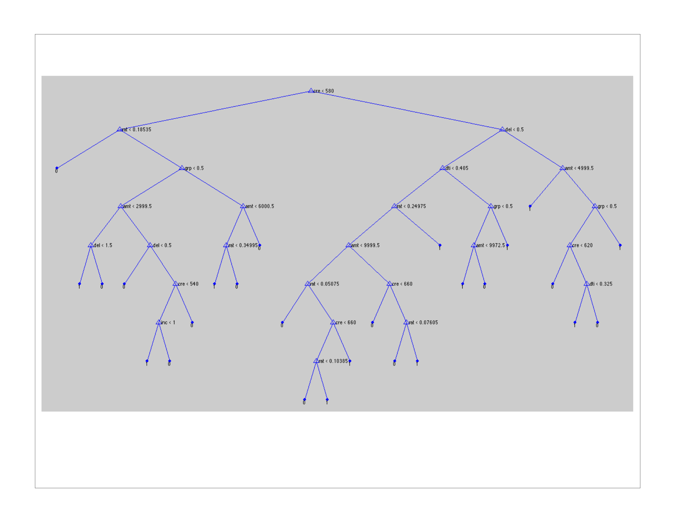
The output file does not transfer well visually; suffice it to say that, given a borrower profile (e.g. B credit score, no delinquencies, debt-to-income 10%, asking for a $1500 loan at 11% interest), one could manually work through the tree nodes to answer the question “is it likely that this person will receive the requested loan?” Note that in this example, the borrower has a greater than 50% chance of receiving a loan; however, one can also infer from the tree that the same borrower with a C credit score would have a less than 50% likelihood of receiving the loan.
We first tested the significance of using prior probabilities, and found the difference was important in the case of loan – no loan and less significant in the case of default - paid. For a 10-feature tree, with a node split threshold of 10, for example, there was an 11-percentage point difference in error rates with and without prior probabilities.
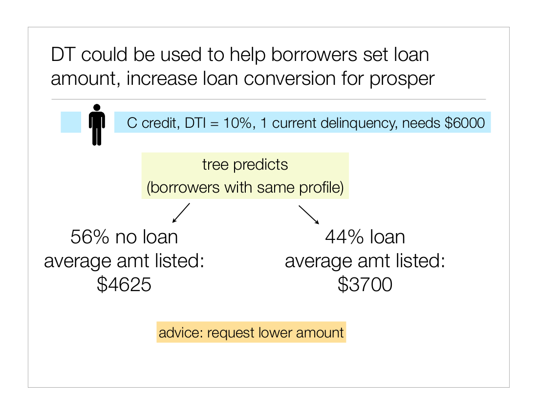
We were particularly interested in the potential applications of decision trees to the judgments made by prosper lenders and borrowers. For example, a prospective borrower might extract probabilities from a decision tree in order to better calibrate his maximum interest rate and loan amount to levels likely to get funded in the prosper marketplace.
The following depiction illustrates how a borrower with the given profile might be advised to lower his requested loan amount (We note in passing that there are two “types” of features: those within and those without the immediate control of the borrower. Features of the first type include loan amount, max interest rate, degree to which profile is filled out. Features of the latter type include credit score, credit history, income, and so forth) Prosper itself has an interest in increasing loan conversion, as the company’s profits are a cut of the total dollars transferred through the marketplace.
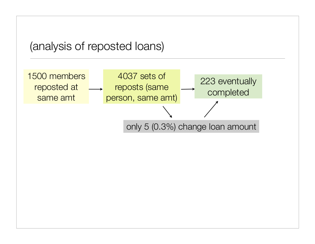
A small side project considered the pattern of re-posted loans in the prosper marketplace. We noted a pattern of many listings from the same borrower that were never converted to loans, and queried for instances in which the same prosper member requested the same loan amount several times in sequence (which we defined as a “repost”; of course, without text analysis it is not possible to know whether the repeat loan at the same price was indeed a relisting of the same loan; we also miss loans in which the borrower changed the amount and only reposted once).
For each of these same member-same amount instances, we calculated the number of “cancelled” “withdrawn” and “completed” loans. The following depiction summarizes our findings: a very small percentage of repeat listings ever get funded, and an even smaller pool of prosper members use the strategy of changing loan amount in order to attempt to get a loan following a failed listing.
We believe this analysis shows the potential for prosper to use predictive models of loan conversion to offer advice to help members convert more listings to loans (of course, this conclusion rests on the assumption that the prosper lending pool is not zero-sum; that is, that with stronger listings more money from lenders would flow into the prosper marketplace).
Analysis of Results
We used training and testing data to quantify the overall accuracy, as well as the sensitivity to different training data, of each of the decision tree models (loan-no-loan and paid-default). Error was calculated as the proportion of mis-classified outcomes in the testing data set.
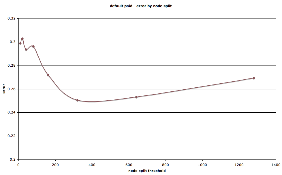
We also conducted analysis to compare trees and find the trees most accurate for each of the two initial problems. First, we varied the node split threshold to find the optimum split level. As with most models, there exists a trade-off between over and under specificity. We found that, for the default-paid question, the sample for node split that minimized error was about 200-300.
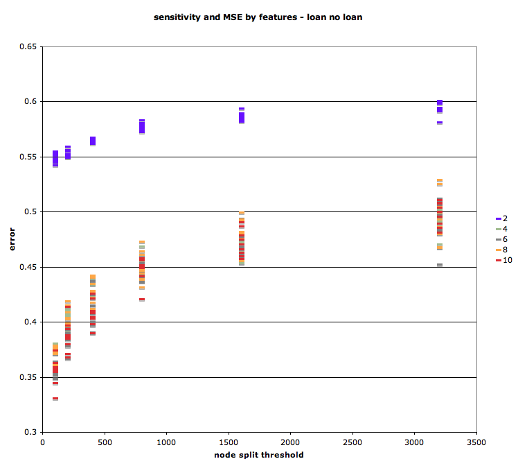
Interestingly, for the loan-no-loan problem, error rates continued to decrease as the node split sample minimum was decreased to just 2 samples. This is probably due to the unequal prior probabilities of the two outcomes: below, we show that depending on what question one hopes to answer, it is possible to calibrate the model to minimize either the false positive or false negative rate.
The tradeoff between overfitting and insufficient granularity
We also considered the number of features that minimized error rates. With just four features (amount requested, maximum interest rate, credit score, income), it was possible to achieve an accuracy of greater than 75% for the loan-no-loan question.
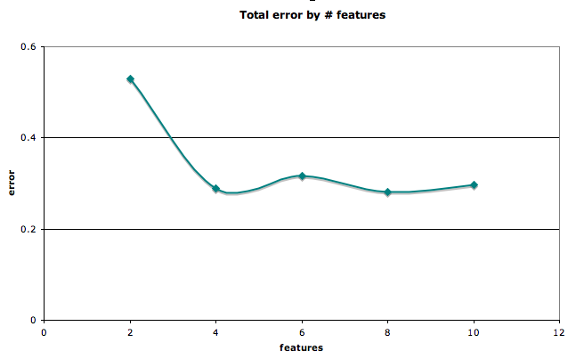
Error rates by number of features for loan/no-loan
Using the holdout sample of 10% testing data, and iterating 10 times, we were able to test the sensitivity of the model to different sets of training and testing data. Generally, as the number of features decreased, the variance of error decreased slightly. Similarly, there was a small decrease in the variance of error as the node split threshold was set higher.
Loan vs. no loan.
As mentioned above, there is a tradeoff between classifying as a loan a listing that doesn’t convert (false positive) and classifying as not-converted an actual loan. In medical decision-making, for example, the trade-off between false positives and false negatives is frequently weighted: one would prefer to over-diagnose a deadly disease, for example, in order to minimize the rate of “misses” or failing to detect the illness in an affected individual.
In the prosper marketplace, the parameters of the tradeoff between false positives and false negatives are not so obvious. We’ll say simply that it is possible to calibrate the model to increase the identification of loans (at the cost of most false positives) or to decrease the number of missed loans (false negatives), by changing the minimum number of samples required to split a node.
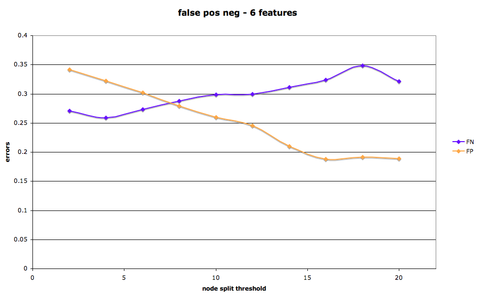
False positive, false negative rates by node spit threshold for loan-no-loan tree.