Baseball Activity and Player Recognition from Inertial Sensor Data

Gershon Dublon and Jared Markowitz

MAS 622J/1.126J

Pattern Recognition and Analysis

Final Project Report

Introduction and Motivation

Baseball is a sport known for the extensive statistical analyses teams employ to gain an edge. Major League organizations spend huge amounts of time and money evaluating player performance through a variety of statistical methods. Similarly they dedicate many resources toward keeping their players healthy, doing everything they can to enable peak performance. To this point there has been relatively little effort to merge the worlds of statistical analysis and sports medicine; in particular there has been relatively little effort expended to quantify the mechanics of baseball movements at a sufficiently high resolution to understand the enormous forces and torques the game exerts on the joints of its players. These quantities are of particular interest to sports medicine researchers who seek to better understand the common causes of injury, catch problematic behaviors before they cause long-term damage, and design safer practice and play guidelines for professional athletes. Beyond sports medicine, researchers are beginning to evaluate quantitative metrics to characterize player performance and skill in order to design of more effective and targeted training regimens.

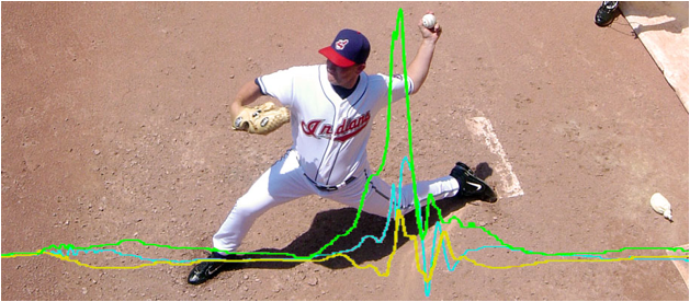
Motion capture systems are the quantitative tools most commonly applied to this problem, but fail to capture the intricacies of player technique. This results from their lack of spatiotemporal resolution and the precise setup and calibration they require, which effectively precludes portability to the ballfield. This project leverages sportSemble, a sensing platform built by Lapinksi et al, of the Responsive Environments Group at the MIT Media Lab [1]. sportSemble consists of a set of small, high-precision, high-range inertial measurement units (IMUs) designed for sports medicine and performance evaluation. The sportSemble system enables high-resolution measurements of the linear accelerations and angular velocities of the relevant limbs and joints, while avoiding the pitfalls of the traditional motion-capture approach.

In this project, we take a first pass at a dataset of professional pitchers and batters, aiming to extract and map a feature space of these data and discover good features for classification of a number of player activities: pitch type, swing type, and the resultant ball locations for pitches and swings. We also report on feature selection and classification of player identification, using the same motion signatures as biometric identifiers. It is worth noting that these problem differ significantly (in data and feature-space) from the classical IMU-centric “activities of daily living” (ADL) recognition problem because the relevant examples are all of duration less than one second and involve accelerations, angular velocities, and fine motor control well beyond most human capability. We select and test features, reporting the results for a number of classification schemes, including naïve Bayes, k-Nearest Neighbor, Linear Discriminants, and Support Vector Machines.

Dataset

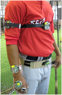
The sportSemble dataset is collected from professional baseball players who are directed to perform common tasks (pitching and swinging). The players wear five 6-degree-of-freedom (6-DOF) IMUs on their hands, forearms, upper arms, chests, and waists. Each IMU consists of two 3-axis accelerometers and two 3-axis gyroscopes (one of each for high- and low-range measurements), as well as a 3-axis magnetometer (which we did not consider) and a radio for synchronization. The data is stored to local flash on each IMU at a sample rate of 1000 Hz for the high-range and 330 Hz for the low-range sensors. Each example includes 8 seconds of data for each axis of each sensor, adding up to slightly under 300,000 data points per example. The labels are annotated during data collection and manually entered into a database (together with the data) later. These data and labels are retrieved from the database as needed.

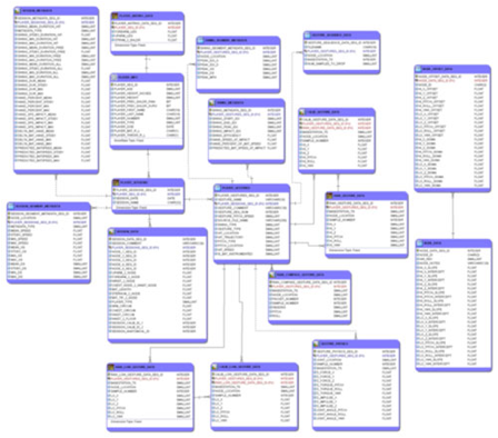
Figure 1: Learning PostgreSQL: the structure of the sportSemble database

For the purposes of classification, there were insufficient numbers of examples for several of the relevant classes. For example, there were only 3 curveballs in the entire set. Since very little can be extrapolated from the correct (or incorrect) classification of such small numbers of examples, we discarded those out of hand (though in clustering and plotting we did find that 2 of the 3 curve ball examples were very close together and extremely far in 3-feature space from any other examples). Data corresponding to unrealistically small classes was retained for the other classification problems if its other labels were sufficient (i.e. curve balls cannot be classified, but their locations can). After a tedious process of weeding out bad (glitchy, missing, unacceptably noisy) data and examples in which the relevant activity is partially cut off in time (either at the start or end of the data), we were left with the following numbers of each motion. The number of examples per class are given below to convey a sense of the baseline (naïve) prior performance we hoped to beat.

Pitch Type	No. Examples	Pitch Location*	No. Examples
Fastball	131	Left	78
Change	39	Middle	114
Slider	9	Right	41
2-seam	17	Top	18
4-seam	7	Middle	139
Break	27	Bottom	76
Total	230	Total	233

Swing Type	No. Examples	Swing Location*	No. Examples
Tee	91	Left	60
Soft Toss	90	Center	76
Normal	33	Right	78
Total	214	Total	214

Table 1: Motion types and number of each that were used in this analysis.

Player ID (pitchers)	No. Examples	Player ID (batters)	No. Examples
#2	22	#1	15
#3	33	#12	20
#4	33	#13	12
#5	36	#15	19
#6	42	#16	17
#8	24	#18	19
#9	21	#21	44
#31	22	#23	14
Total	233	#24	15
		#25	18
		#27	21
		Total	214

* Location labels were flipped for left-handed pitchers and batters so as to be symmetric with respect to the IMU axes on the right-handed players.

Table 2: Player ID labels and numbers of each for pitching and swinging

Procedure

1.) From the raw data described above, we extracted 196 pitching features and 200 batting features.

2.) Several methods of feature selection were considered to determine the features relevant to several different classification problems. Sequential Forward Selection was used to determine final features.

3.) The performances of four classification schemes (NB, kNN, LDA, SVM) were evaluated and used to improve understanding of the data set.

1. Feature Extraction

Extracting good features from the data was a challenge because there is a large amount data per example. It is not immediately obvious which data is most relevant for the extraction of salient features, and what the most salient features are. For pitchers, we used the high-range (higher sampling rate, lower bit depth) sensor data for the hand, forearm, and upper arm, and low-range (lower sampling rate, higher bit depth) for the waist and chest. For batters, we used the high-range sensor data for the hand and forearm, and low-range for the upper arm, waist and chest. These choices reflect the magnitude of the motion recorded at each IMU, which saturates the low-range sensors on all the players’ hands and forearms, and on pitchers’ upper arms.

i. Peak timing

Given the peakiness of the raw data and relatively short time spans involved, we hypothesized that relative peak timing between axes and across IMUs would be most salient for our classification problems. We encoded this feature by defining an “origin” for each pitching example to be the highest peak in the z-axis of the hand (pointing out in the direction of the hand), consistently the highest and sharpest peak. The origin for each batting example was given by the impact time, a pre-computed feature by Lapinski, et al. Once the origin sample index was extracted, we extracted the 2 highest peaks from each remaining IMU (accelerometer and gyroscope) axis and retained the time between those peaks as features.

ii. Relative peak heights and inertial magnitudes

We extracted the heights of the 2 highest peaks of the rectified signal in each axis and from the IMU magnitudes of acceleration and rotation. We then “normalized” these values by the height of the highest peak in the data (hand acceleration in the z-axis) in an attempt to make the features more invariant to overall player strength. These relative peak heights were recorded as features.

iii. Spectral peaks

We computed a zero-padded, 1024-point Fast Fourier Transform (FFT) for each axis, and retained the frequencies corresponding to 3 peaks in the spectrum for those signals that had periodic characteristics. For example, the hand acceleration in z had no peaks in the spectrum (as it is an impulse in time), while the x and y axes in that IMU tended to have clear spectral peaks.

iv. Full-width at half maximum (FWHM)

We computed the full duration at half-maximum of the highest peaks of the magnitudes of acceleration and rotation in each IMU, intended to encode the sharpness of the peaks.

v. Impact timing

We used pre-computed start, impact, and end times provided by Lapinksi, et al. for the batting data, stored relative to impact time. The resulting two features encode the point in the swing when the ball is hit, which is presumed relevant for ball location.

A table of contents of features for pitching is linked here:

Pitching Features

A table of contents of features for batting is linked here:

Batting Features

Feature Selection

The above methods of feature extraction produced very large number of features for each movement, relative to the number of example, almost one-to-one. We tried a number of methods to avoid overfitting and other pitfalls of huge feature spaces.

i. Principal Components Analysis

First, to get a sense of the variance in the feature space, we computed its principal components. Principle Component Analysis (PCA) uses an orthogonal transformation to produce linear combinations of the original features that are uncorrelated, with the resulting components being listed in order of decreasing variance. This analysis exposes the correlation between features, and shows where the variance of the feature space is concentrated.

Results of this step are shown in Figure 2 which shows that the dominant components best separate individual players (as opposed to classes), indicating that the features of highest variance vary significantly more across individuals than across motion classes. Indeed, only 2 components account for 93% of the variance in the set. These results were initially discouraging, though they suggested immediately that certain features that are especially good for separating players would not be good, and that variance in the feature space is not necessarily a good indicator of goodness.

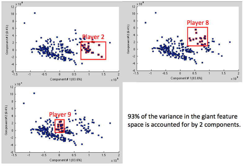
Figure 2: First two components of PCA account for almost all the variance in the feature space, and separate players into clusters

ii. Mutual Information

Several techniques were then applied to determine which individual features are most closely linked with labels. The labels we refer to here are pitch type and pitch location, hit location, and player ID. To start, we first computed the mutual information, I(X; Y) of each feature X with each output label Y.

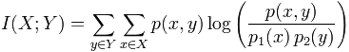
Mutual information measures how much the distributions of the variables differ from statistical independence, and thus here measures the dependence of the output label with each individual feature. An example plot of how mutual information varies across the features is shown below. While mutual information does give a sense of how much the output is correlated with each input, it does not consider potential interaction between features in producing an output and hence is not an ideal feature selector. Still, the distinguishable peaks in this quantity indicate features that are correlated with the labels. Figure 3 shows more variation and peakiness in the mutual information for pitch type than hit location.

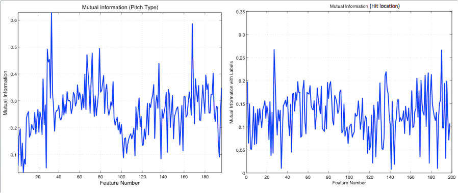
Figure 3: Mutual Information vs. Feature Number for pitch type and hit location

iii. Sequential Forward Selection

To better understand how the interactions between features affect the output labels, we proceeded to apply a Sequential Forward Selection (SFS) algorithm to select features. Such an algorithm is based on the accuracy of an individual classification method on predetermined subsets of the data (training and testing sets). The algorithm proceeds in a “greedy” manner, starting with no features and then keeping the feature that most improves the classification accuracy in each run through the data. The algorithm can be terminated at either a predetermined number of features or once the addition of another feature yields only a small increase in performance. In this study SFS was applied with 3 different classifiers (NB, kNN, LDA) with varying success, as described below. The classification performance was evaluated using both the leave-one-out and 10-fold cross-validation methods for dividing the data into training and testing sets. The leave-one-out method selects a single example for classification, using the rest of the data set for training. This process is repeated for all points in the set, and an over-all accuracy is then computed. The 10-fold cross-validation method randomly partitions the data set into 10 subsets and then, for each subset, classifies the points using the other 9 subsets as training data. The overall accuracy of this method is then the classification accuracy over all 10 subsets. The performance of the 10-fold cross-validation is likely to be more realistic (or is less likely to overfit) than leave-one-out as it relies on less training data for each classification and does not have an individual training set for each point. Below we discuss the results of this classification scheme for each of the different classification problems and classifiers that were pursued in this study.

Classifiers

i. k-Nearest Neighbor (k-NN)

In this classifier, a given point is classified according to the classes of the k training samples nearest it in the feature space (here the Euclidean distance is used). The point in question is sorted into the class that contains the largest number of the k surrounding points. The kNN algorithm works well on data sets where the classes are distributed in largely homogeneous clusters (including those with multiple clusters per class).

ii. Naive Bayes

The Naive Bayes classifier assumes that the value of a given feature is conditionally independent of that of any other feature, given the class. The classifier then chooses the class with the highest conditional probability given the feature observations, based on the training set.

iii. Linear Discriminants (LDA)

Linear discriminant classification learns the linear combination of features that best separates the classes in the feature space. In general, linear classifiers work best separating classes that are not distributed in clusters throughout the feature space, but easily separated by hyperplanes. LDA performance can often be improved by combining weak-performing linear classifiers through Adaptive Boosting or other meta-algorithms.

iv. Support Vector Machines (SVM)

At the most basic level, SVM classifiers find a separating hyperplane in the feature space, similar to the LDA classifier. In contrast to LDA, SVMs can map the feature space to a higher dimensional one, such that classes that are not linearly separable in the original feature space become separable in the new one. In particular, SVMs with radial basis function kernels are well suited to feature spaces where a single class is divided in the space by another, because they bend the space along the line joining the separated class clusters to join the class before applying the separating hyperplane. This principle is further elucidated below.

out

Results and Discussion

The results of the Sequential Forward Selection (SFS) algorithms used here are displayed in Tables 3, 4 and 5. Six different classification problems were analyzed: pitch type (fastball / changeup / slider / two-seam fastball / four-seam fastball / breaking ball), pitch horizontal location (left / right / center), pitch vertical location (up / center / down), pitcher identification, hit direction (left / center / right), and batter identification. Table 3 and Table 4 show the results using leave-one-out and 10-fold cross-validation for choosing training and testing sets. It should be noted that the selection applying leave-one-out cross-validation always tried up to 20 features and picked the number with the best classification accuracy, while the selection using 10-fold validation stopped as soon as the addition of one feature failed to improve classification accuracy. 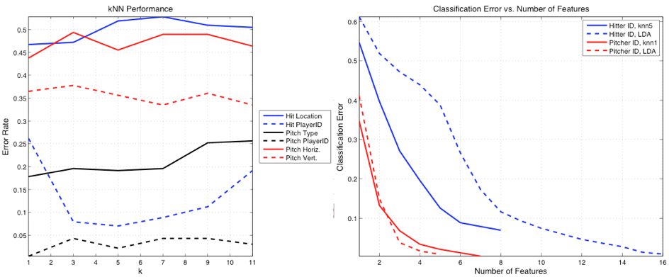Five different values of k in the k-NN algorithm were tested in each case, with the best k being reported in the tables. As shown in Figure 4 (A), the classification accuracies in most problems did not change appreciably for k varying from 1 to 11 (with the exception of the batter identification problem). Figure 4 (B) shows the convergence of the errors in the player ID problem using the LDA and k-NN classifiers.

Leave-one-out Cross-Validation

Class. Problem	Method	# Features	Top 10 (or less) Features	Error
Pitch Type	kNN5	4	29,79,33,66	0.1803
Pitch Type	LDA	1	141	0.5107
Pitch Horiz.	kNN9	8	165,34,109,159,67,123,56,126	0.382
Pitch Horiz.	LDA	4	43,4,138,29	0.4721
Pitch Vert.	kNN3	2	148,85	0.3777
Pitch Vert.	LDA	1	138	0.4421
Pitch Player ID	kNN1	8	68, 153,96,31,24,60,97	0.0043
Pitch Player ID	LDA	4	61,174,180,53	0.0086
Hit Direction	kNN3	4	50,143,62,128	0.5047
Hit Direction	LDA	4	28,84,60,6	0.5093
Hit Direction	NB	3	179,138,121	0.5561
Hit Player ID	kNN1	8	79,57,93,89,55,125,134,128	0.0467
Hit Player ID	LDA	9	57,89,59,79,173,189,82,188,61	0.0187

Table 3 : SFS results using leave-one-out cross-validation and kNN, LDA, NB classifiers.

10-fold Cross-Validation

Class. Problem	Method	# Features	Top 10 (or less) Features	Error
Pitch Type	kNN1	7	29,33,58,65,67,79,89	0.1783
Pitch Type	LDA	6	7,29,115,141,142,167	0.4739
Pitch Horiz. Loc.	kNN1	4	8,71,84,105	0.4378
Pitch Horiz. Loc.	LDA	2	43,138	0.4893
Pitch Horiz. Loc.	NB	3	77,130,196	0.4635
Pitch Vert. Loc.	kNN7	3	57,82,153	0.3348
Pitch Vert. Loc.	LDA	1	138	0.4549
Pitch Vert. Loc.	NB	3	68,77,128	0.3605
Pitch Player ID	kNN1	8	55,57,65,66,67,126,144	0.0701
Pitch Player ID	LDA	5	47,61,136,174,180	0.0093
Hit Location	kNN1	5	27,46,53,96,125	0.4673
Hit Location	LDA	2	28,84	0.5234
Hit Location	NB	2	89,95	0.5794
Hit Player ID	kNN5	8	55,57,59,79,89,91,93,167	0.0701
Hit Player ID	LDA	16	15,17,51,53,57,58,64,73,87,122	0.0093

Table 4: SFS results for best kNN, LDA, and NB using 10-fold cross-validation.

Class. Problem	Method	# Features	Top 10 (or less) Features	Error
Pitch Type- FAST	SVM	2	141,168	0.2696
Pitch Type-CHANGE	SVM	2	27,184	0.1391
Pitch Horiz. Loc. - L	SVM	2	27,82	0.2935
Pitch Horiz. Loc. – C	SVM	2	4,63	0.3312
Pitch Horiz. Loc. – R	SVM	3	63,84,115	0.1438
Pitch Vert. Loc. –HI	SVM	2	105,136	0.0594
Pitch Vert. Loc.- MI	SVM	4	58,104,139,146	0.3215
Pitch Vert. Loc.- LO	SVM	5	56,92,108,120,154	0.2489
Hit Location – L	SVM	1	103	0.3076
Hit Location – C	SVM	4	16, 58,122,146	0.2394
Hit Location - R	SVM	3	131,136,148	0.3112

Table 5: SFS results for SVM classifier using 10-fold cross-validation. Results are omitted for the smallest classes due to overfitting.

Figure 4: (A) k-NN performance versus k. (B) Reduction of error with number of features in SFS.

Several features of tables 3,4 and 5 stand out. The majority of the features chosen by SFS relate to the timing of the accelerometer and gyroscope data on the hand and forearms, confirming expectations given the motions recorded. The exceptions to this trend are the player ID classification problems, where measurements taken at the waist and upper arm are found to be more important. One explanation for this would be that the differing body structures and strengths of the different players could be used to identify them and would be better reflected in the data from these proximal sensors. Overall, many different features were found to be relevant depending on the problem and the approach. Given the redundancies in our “kitchen sink” approach to feature extraction, this is not an unexpected result; however, the small size of the dataset relative to the feature space significantly increases the risk of overfitting. We clearly saw these effects on the smallest classes, and especially given the binary training and classification of SVM. For example, SVMs achieved a 1% error rate after feature selection on the pitch type slider (with only 9 examples in the set), and 27% error for fastballs (which account for half the dataset). As a result, we omit from this report the results of feature selection using SVM for the smaller classes, which can only be accounted for by overfitting. On the bright side, the feature selection framework is in now in place to accept more data, which would allow us to draw more conclusions about SVMs and limit these effects.

Player ID for both pitchers and batters proved to be by far the easiest classification problems to solve, with less than 1% error for the 1-NN classifier in 10-fold cross-validation, using as few as 5 features. Figure 5 shows why this is the case, namely that the points for individual players appear to be separated into player-specific clusters. As is detailed below, this is because the feature space points appear to be more homogeneously clustered by player than by motion. As far as methods go, it is apparent that the performance of k-NN and SVM consistently exceed that of LDA and NB. The LDA classifier was ineffective because there were often multiple clusters representing each class that were interspersed in feature space, making it impossible for a linear discriminant to separate them. The weak performance of Naive Bayes was likely due to the fact that the distributions of different features were not independent, as is to be expected given the mechanical relationships among the various extracted features.

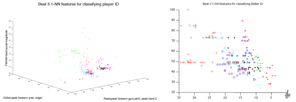
Figure 5: Player-specific clusters are clearly separable for both pitchers and batters

Figure 6 shows all the examples plotted in the 2-d space of the best features selected for 1-NN classification of pitch type, the relative timing of peaks in hand gyroscope yaw and hand gyroscope pitch. The figure indicates that the largest class in the dataset, fastball, is separated in feature space by another class, breaking balls, suggesting that SVMs should perform better than the other classifiers. As noted above, feature selection for the binary classifier SVMs was a challenge due to overfitting on the smallest classes. As a result, to further explore the potential of SVMs without exposing the method to the same level of risk of overfitting, we trained SVMs on the top 20 features selected for 5-NN classification, hoping that features selected by a classifier considering the entire space of classes might be less prone to overfitting. Note that these results should not be directly compared with the results above because the SVM method used different feature sets for each of the binary classification problems it examined.

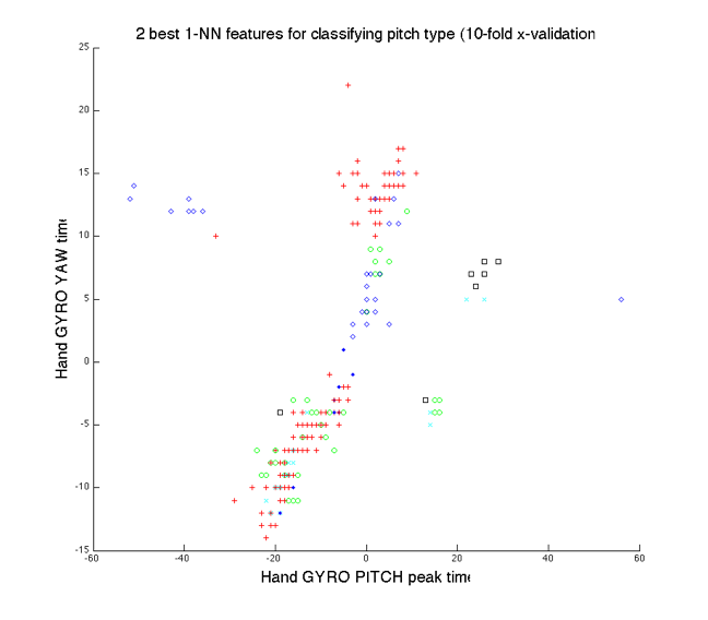
Figure 6: Fastball class is clearly separated by breaking ball class

Using the k-NN feature set, SVMs out-performed the other classifiers we tried, without having run feature selection specific to that classifier. We trained SVMs to classify pitch type using the features selected by the SFS for a 5-NN classifier, and applied leave-one-out cross-validation to test their performance. The performance far exceeds that of a naive classifier, especially for the smallest classes, and would almost certainly benefit from more data for those classes. Table 5 shows the performance compared to the distribution of examples. Though we cannot conclude much from this limited test, we believe the results would improve for the smaller classes if we had more data to describe them (training and testing with fewer than 10 examples per class is not ideal). We used the publicly available LibSVM to conduct these tests [3].

Class (distribution of examples)	SVM Performance (true positives)
1. Fastball (57% of set)	85%
2. Change: (17% of set)	64%
3. Slider: (4% of set)	45%
4. 2-seam: (7% of set)	30%
5. 4-seam: (3% of set)	58%
6. Break: (12% of set)	70%

Table 5: SVM compared to prior distribution of classes.

Varying the cost parameter for the SVM, which varies the softness of the separating hyperplane, we found that a lower cost would result in better performance on the largest class (fastballs), especially as it relates to the rate of false positives, which increases with fuzzier separation.

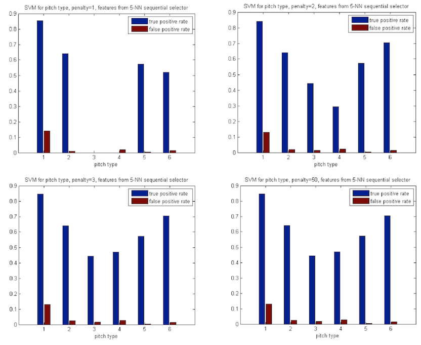
Figure 7: Lower SVM cost parameter results in better performance on the larger class, worse performance for others.

Conclusion

The relative performance of the different classifiers indicate a feature space in which the variability between players is larger than the variability between motion types. We believe that the performance of k-NN and SVM and the complete failure of LDA and NB is due to the arrangement of the feature space, in which the large separation due to subject variability fractures the distributions of different motion types. K-NN and SVM are far more invariant to this kind of arrangement than linear and Naive Bayes classifiers, which struggle to linearly separate the classes. We theorize that data from players with similar techniques (that result in close proximity in the feature space) would be easier to classify based on motion type. Indeed, the clear division of the fastball class into two distinct large clusters (as shown in figure 6) may be due to a dichotomy in subject technique. With more data, similar player types could be identified and investigated in separate groups.

Summary

We applied a set of pattern recognition algorithms to a new dataset of professional baseball players performing activities such as pitching and batting in an attempt to classify common techniques for those activities. We found that these data almost perfectly separate individual players, but struggle to distinguish amongst player activities. We suggest ruling out LDA and NB, and focusing on those classification techniques that can better handle fragmented class distributions.

Future work

There are many ways that the study presented here could be improved and extended. The first and obvious way to improve the results would be to obtain a larger data set, particularly since there are currently only a few examples of several of the classes. A larger data set would allow us to more reliably train our classifiers. The data itself may also be improved through the use of more careful methods for classifying pitch type, as there are believed to be some misclassified pitches in the database.

More sophisticated feature selection means could also be implemented. The current SFS method of selecting features could be improved upon by implementing a Sequential Forward Floating Search algorithm (SFFS). Such methods are not “greedy” in that they can improve performance by backtracking, thereby reconsidering features that could have been erroneously added or removed. One could also look at implementing backwards feature selection algorithms (SBS, SBFS), where the classification performance is evaluated while features are sequentially removed from the full feature set rather than added to an initially empty feature set. One drawback of backwards algorithms is that they are typically more computationally expensive than their forward counterparts. This could be alleviated by using a forward algorithm to first eliminate some features that are clearly unimportant and then implementing the backwards algorithm on the remainder. In all these classification methods, it may be useful to try a “Leave One Player Out” means of dividing the data set, given the strong player-based clustering observed here.

In this work, we began looking at boosting the linear classifiers, without much success, though further investigation is warranted. Separately, given the results we obtained, a Decision Tree classification scheme may be worth considering. In this approach, grouping of players with similar characteristics could represent the first division. In general, cascading linear classifiers could avoid some of the pitfalls we encountered using LDA.

Additional classification algorithms, particularly temporal methods, could potentially shed more light on this data set. Temporal methods could be implemented by windowing each data series and looking at how features change throughout a motion. This could be used to train a Hidden Markov Model (HMM), for example, which progresses through hidden states as time evolves. It would be particularly interesting if such a model was found to correspond to states that coincide with the accepted biomechanical phases of pitching and hitting.

Finally, there are many more questions that can be asked using this data, and many other ways that it could be applied. As seen above, individual players tend to cluster strongly in some feature space. This observation could be used to explore player similarities and potentially determine features that identify different groups of players (those that are successful, those that are injury prone in a particular way, etc). Another class label that could be explored is player fatigue, which would be indexed simply by the timing of a gesture in a data session. One could look at the changes that occur in features as a player tires and classify fatigue levels based on this information. This has obvious sports medicine implications, as it could help explore potential sources of injury as a player tires.

Figure 7: Fortune cookie (from 12/9/10) confirms that 42.7% of all statistics are made up on the spot.

Code

Download our Matlab code at:

http://www.media.mit.edu/~gershon/MAS622j/final_project/code.zip

References:

[1] Michael Lapinski , A Wearable, Wireless Sensor System for Sports Medicine, MS Thesis, MIT Media Lab, September 2008

[2] Richard O. Duda, Peter E. Hart, and David G. Stork, Pattern Classification. New York, NY: John Wiley & Sons

[3] Chih-Chung Chang and Chih-Jen Lin, LIBSVM : a library for support vector machines, 2001. Software available at http://www.csie.ntu.edu.tw/~cjlin/libsvm