Magnetic Localization
by Matt Donahoe
 | The ProblemGPS technology has enabled many interesting and helpful applications, but unfortunately it only works reliably when the user is outside. In this project I am investigating the effectiveness of magnetic field sensing for indoor localization. The earth's magnetic field is mostly uniform when measured outside, but inside a steel building the field can be significantly distorted. These distortions are stable and can provide identifying features to different parts of the building. By first mapping out the field distortions inside a building, we can use that map later to guess our location given a magnetic measurement. The purpose of this project is to develop an reliable pattern recognition algorithm that can compute these localizations. |
 | The DatasetThe data for the project was provided by Jaewoo Chung of the Speech+Mobility Group. Jaewoo is working on an indoor navigation project known as Guiding Light, and is testing the use of magnetic field localization. He has built a device with 4 magnetometers and taken data over several paths through the Media Lab. To collect data, he measured the magnetic field around a point in the building. By quickly measuring the field in all directions in the area around a point, he creates a "signature" of that point. This allows that us to recognize that point without having to spend much time accurately measuring the magnetic field. Each point has 100 feature vectors, each with 12 elements |
 | Training DataHe collected "signature" measurements at 300 points along a circular route through the buiding. Each point has its own signature. This becomes the training data. |
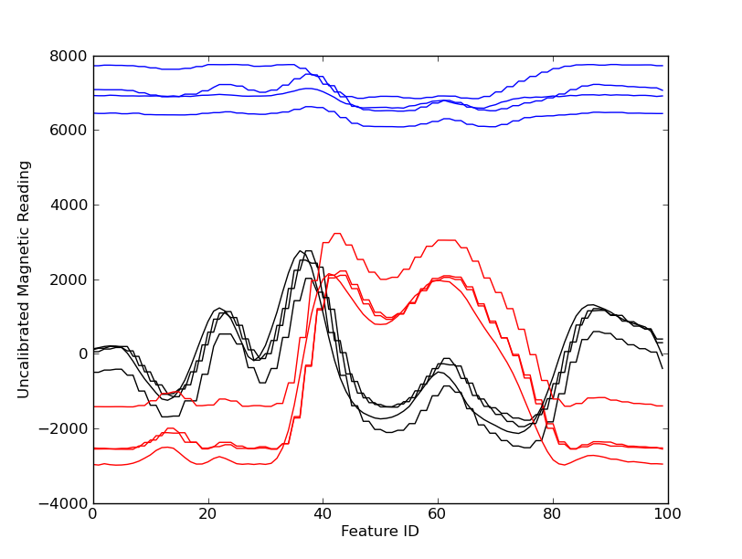
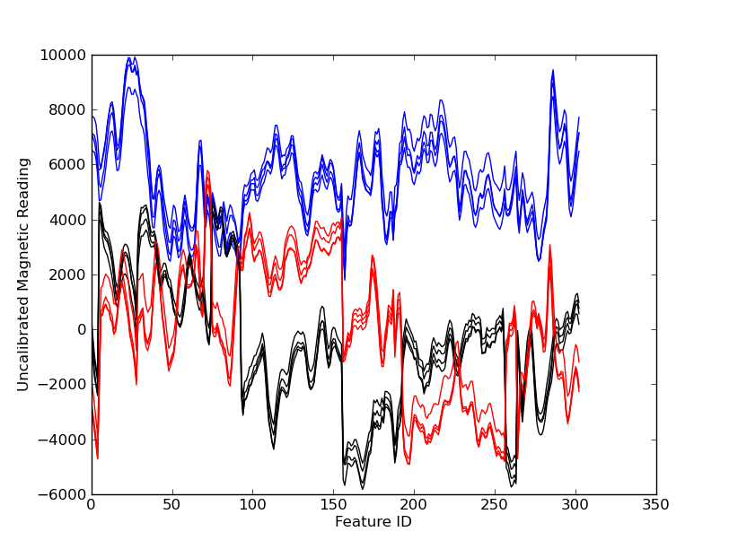 | Test DataFor the test data, instead of taking a measurement in all directions, we only need a single measurement from any direction. We took single measurements at each point in the loop. The goal is to use this samples to predict our location. The plot shows how the feature vector changes as you move through the the building. |
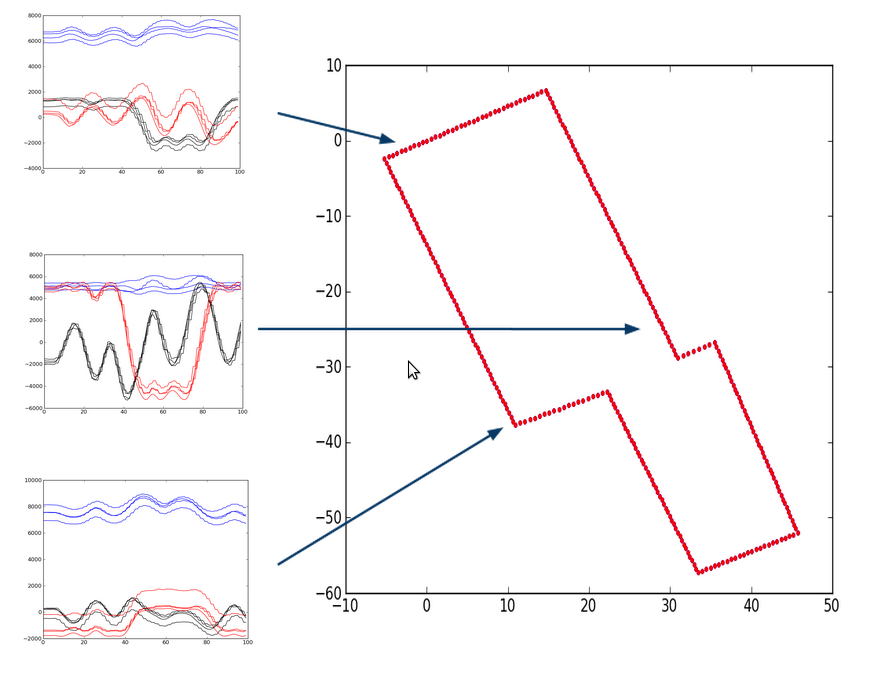
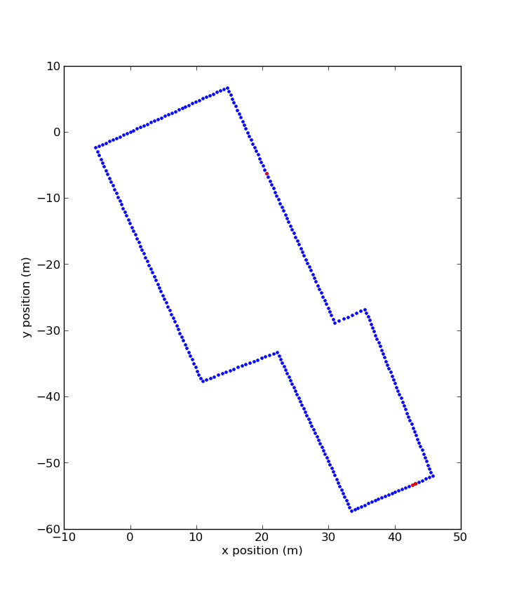 | Similar PointsTo find the correct point given a measurement, we calculate the euclidean distance between the measurement and all the feature vectors in our training set. This is a simple Nearest Neighbors algorithm can yield the correct position given a magnetic reading, but it can also match points that are far away. This map shows the top 3 positions that match a given magnetic measurement. One point is about 40m away from the other two. |
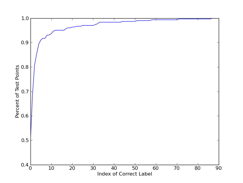 | If we run Nearest Neighbors over the entire data set, we find that 50% of the points are correctly identified by their nearest neighbor. 90% of the points are identified by a one of the top 3 neighbors. However, because the nearest neighbor can end up being a point from accross the map, the mean error in prediction distance is 8m, with a stdev of 16m. |
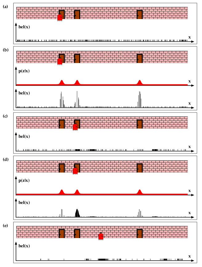 | Particle FilterTo improve upon Nearest Neighbors, we can combine information from successive samples to rule out the outliers. At first I thought of using a Hidden Markov Model to approxmate the position over time, but instead I used a Particle Filter. Particle filters are similar to HMMs in that they both attempt to guess a hidden state based on observation data, but whereas HMMs use a network model with discrete states, Particle filters use a continous state variable. For example, imagine a robot that is moving down a hallway. We can model its position as a continous state variable x. Let's say we can't measure x directly, but the robot is equipped with a door sensor. When the robot senses a door, it can look at a map of the hallway and guess where it is. a. Before the robot takes any measurements, it could be anywhere in the hallway. That means that the probability is evenly distributed over the possible x values. x is a continous quantity, but for a computer to respresent its values, the space needs to be sampled. To do this, we create N "particles" to represent the distribution. Each particle has a position and a probability. At first, we create N evenly distributed particles with equal probability. b. When the robot takes a measurement, we multiply the the probability of the particle by the probability of seeing that measurement given particle's x position. This changes the probability of the particles, making some more probable that others. c. After updating particles, we can resample the distribution, removing particles that have low probabilities and duplicating particles with high probabilities. Additionally, if the robot moves, the particles must move as well, according to a probabilistic model of the robot's motion. For example, if the robot moves forward 1m, the particle motion model might be xt+1 = xt+ 1 + N(0,0.1). The noise term represents the uncertainty in the motion model. This image is from "Probabilistic Robotics" by Sebastian Thrun |
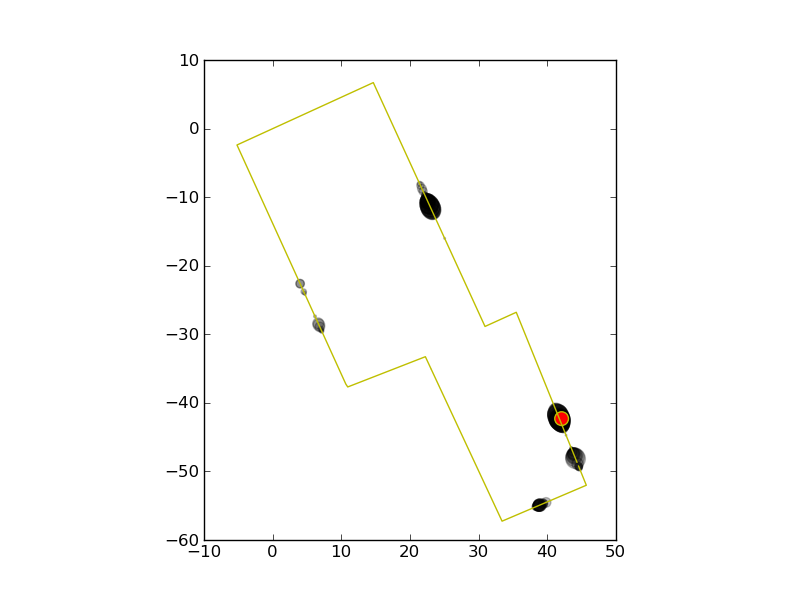
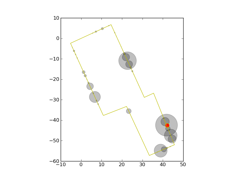 | For our problem, instead of a door sensor, we have our magnetic measurements. First we spread 1000 particles evenly over the entire loop. After the first measurement, a number of particles become very likely, while most of the rest become unlikely. The red dot is the actual position |
 | The particles are resampled and then moved according to the motion model xt+1 = xt+ N(0,1). |
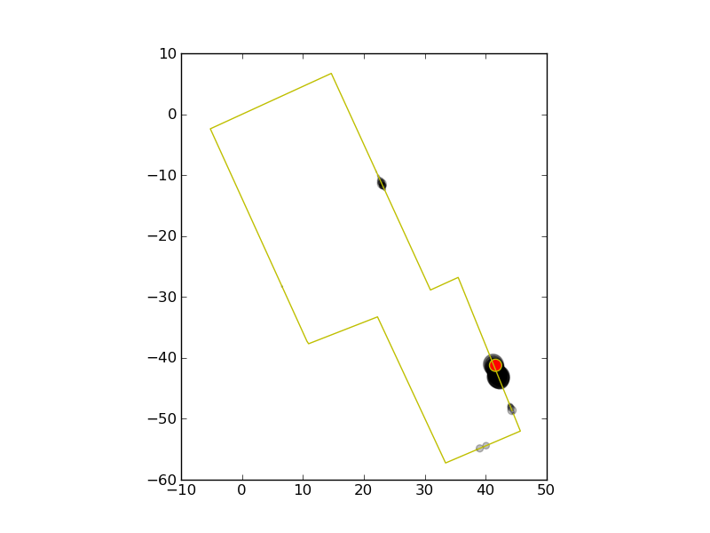 | Each additional measurement causes the distribution to shrink. |
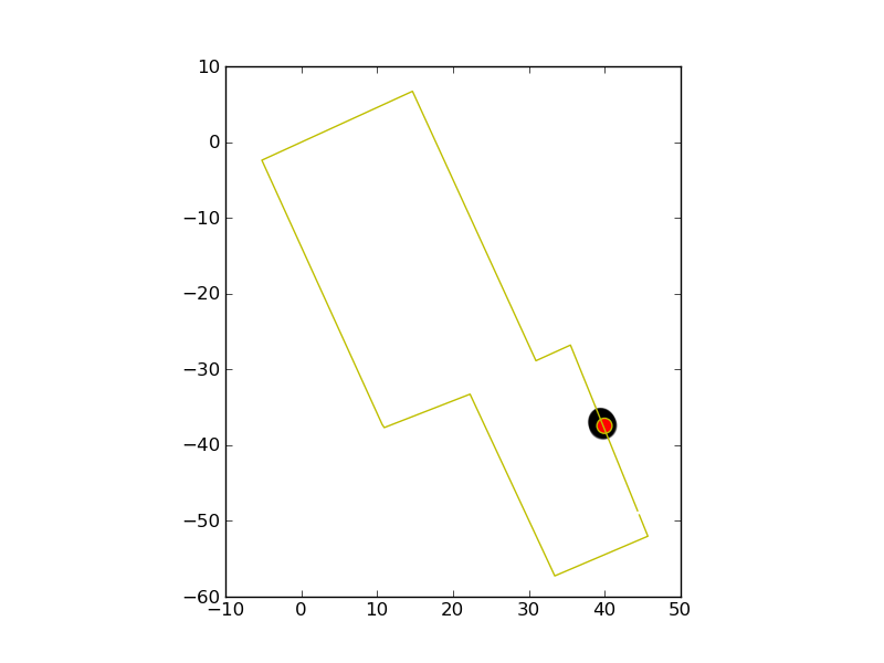 | After a few samples, we have a very confident measure of our position |
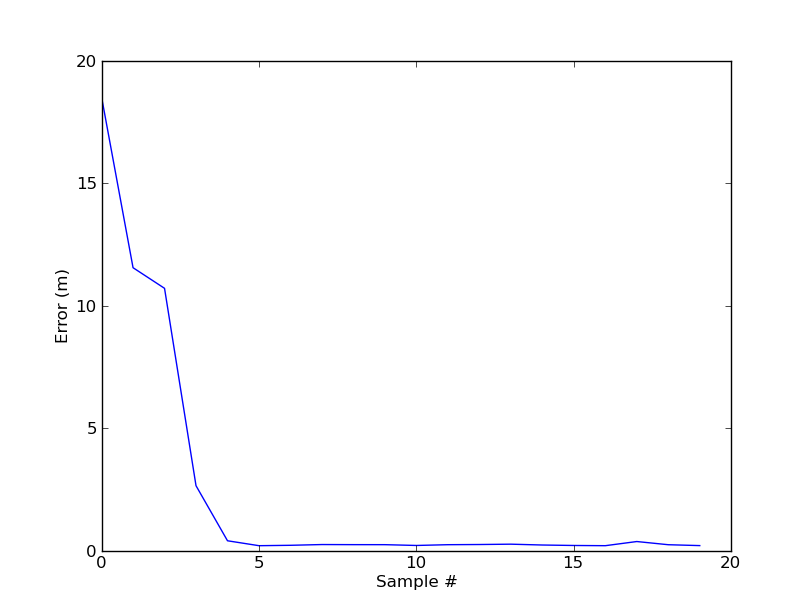 | The error over the time drops quickly which each sample. |
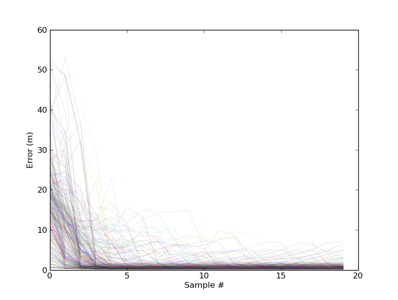 | The ResultsOver the entire test data, we find that most trials have similar behavior. The average error after 20 samples is 0.7m, with a stdev of 0.89m. From the graph you can see there are a few outliers where the particle filter got offtrack, but the max error was only 7m, which is still better than the 8m for Nearest Neighbors |
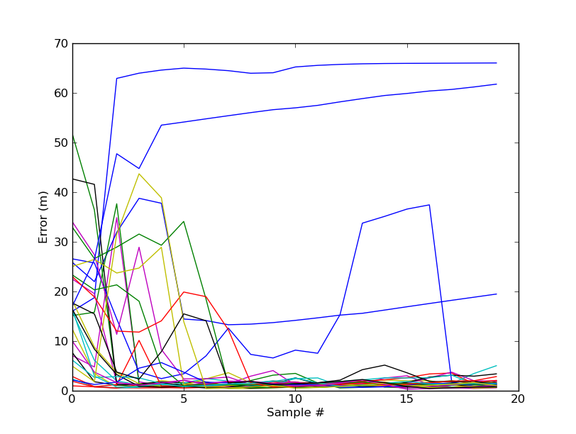 | Fewer Test PointsI tried running the algorithm with fewer training points (75 instead of 300). In the plot you can see several outliers where the algorithm completely failed to track, resulting in position errors of up to 65m. Without these outliers, the average accuracy was 1.5m, which is actually smaller than the distances between training points (3m). |
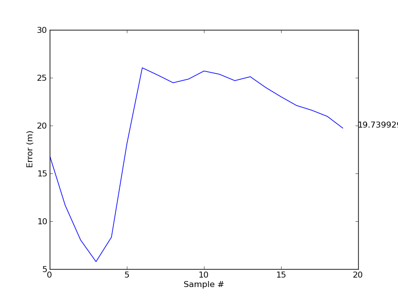 | Magnitude OnlyAlso tried using a smaller feature set. Instead of the representing each position with 100 feature vectors, each with 12 elements, I represented each point with a single average magnitude. This is a significant reduction in data, so I'm not surprised that the results were very unreliable. It seemed that the particles would track for awhile, but could easily get sent off course. Here is a graph of error that changes wildly as more samples come in. |
Basic pseudo code for the particle filter
for each measurement, z:

     scores = the euclidean distances between z and each 12 element feature vector in the training data

     for each particle p:

          #update the particle's probability given this new measurement

          p.prob = p.prob * score_function(scores,p.x)

          #update the particle's position

          p.x = p.x + N(0,1)

     renormalize all particle probabilities to sum to 1

     position estimate = sum([p.prob*p.x for p in particles])


def score_function(scores,position):

     Since the particles are continuously distributed, but the training points are discretely distributed,

     I interpolate the scores for positions that are between points.

     The result is then fed through a gaussian.
Model Parameters
There were 3 model parameters for the particle filter.- The number of particles: (The higher the better)
- Sigma for the motion model: I wanted the particles to move randomly, with a stdev of 1m. The test data points were about 0.6 meters apart. Tuning this parameter would just make the model too overfit to this test set rather than actual walking behavior.
- Sigma for the score function: To make the particle filter work, I needed a way to approximate the probability of seeing a magnetic measurement at a certain position in the building. I used a gaussian to covert the euclidian distance metric into a "probability". The sigma for this gaussian was tuned to produce the best results. I used a seperate test set to do the tuning.
| Sigma | Mean Error (m) |
| 100 | 3.2 |
| 500 | 0.5 |
| 1000 | 1.5 |
| 2000 | 13.8 |