Facial Feature Recognition and the use of Synthetic Training Data
by Derek Eugen Lyons and Larissa Welti-Santos
dlyons@media.mit.edu, lwelti@media.mit.edu
MAS 622J/1.126J: PATTERN RECOGNITION AND ANALYSIS, MIT
This page provides additional detail to support the presentation pages for our final project. Please refer to the linked presentation pages for the large-scale "narrative" behind the project, and refer to this page as needed for more detailed analysis and information.
The dataset for this project is a database of approximately 4,000 face images collected from a broad range of subjects at the MIT Media Lab. The data is labeled according to the sex, race, age and expression of the subject, as well as the presence of any ''props" such as hats, glasses, and facial hair. While the data is not rigorously normalized, it is generally consistent with regard to the eye-location and distance of the subject [2]. For a more complete description of the data, go here.
"Bad" Faces in the Original Data
Besides the faces which were marked as missing from the dataset, a small set of additional faces was found to be unusable for analysis.
Two faces (2412 and 2416) were photographed at higher resolution than the rest of the dataset, and consequently had higher dimensionality. It was also determined that there was no actual data present for 22 faces in the dataset (e.g. the "images" consisted of all 0 values). The offending faces were numbered 2099, 2100, 2101, 2104, 2105, 2106, 3283, 3860, 3861, 4125, 4136, 4146, 4237, 4267, 4295, 4335, 4498, 4566, 4679, 4710, 4779, 4992, and 5113.
In order to focus on pattern recognition (rather than, say, image processing) we deliberately used simple, image-based features to drive our classification. In particular, we follow Belhumeur et al [1]. in the use of Fisher projection coefficients as our features. We will now briefly consider how these features were extracted from the raw data.
Feature Extraction Step 1: Dimensionality Reduction with PCA
Since the raw data had an initial dimensionality of 16,384 x 1, a dramatic dimensionality reduction was a critical first step in feature extraction. Our initial dimensionality reduction was accomplished using Principal Components Analysis (PCA) over the complete training set. In particular, we projected the data onto the 200 eigenvectors of the training set with the largest eigenvalues.
Why 200 Eigenvectors?
Figure 1 presents a plot of the cumulate sum of eigenvalues as a function of the number of eigenvectors.
Fig. 1.
As the figure shows, the eigenvalue sum indicates that 95% of the variation in our training set is accounted for by the first 200 eigenvectors. The remaining eigenvectors correspond to only a tiny percentage of the variation in the training data; this residual variation is likely to be due to noise in the images, and therefore not useful for classification. Thus, we perform our PCA projection onto the first 200 eigenvectors only.
Feature Extraction Step 2: Fisher Projection
Once the PCA projection was completed, we extract our final features by performing a Fisher Projection on the PCA coefficients. A different Fisher projection was computed for each of the features.
Assumptions
When applying PCA and the Fisher Projection, we have assumed that the weak normalization of the position / alignment of the faces was sufficient. We did not use any method to pre-process the original data.
Rather than focusing on one particular classification technique, we elected to try a selection of different methods; the particular method applied to a given feature was determined by the characteristics of the training data. Figure 2 illustrates the process that we followed in order to find the technique which was most likely to be appropriate for each classification task.
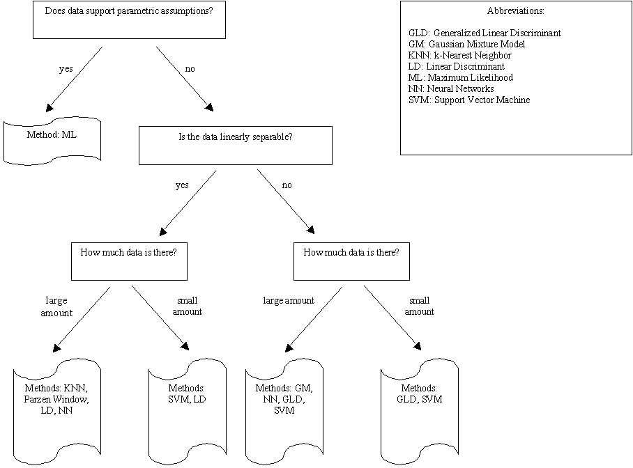 |
Fig. 2.
Of the techniques listed in Fig. 2, we had occasion to utilize maximum likelihood estimation, generalized linear discriminants, neural networks, and support vector machines. We will now briefly describe each of these classification techniques, and our reasons for employing them.
This method seeks parameter estimates which will maximize the likelihood function for the parameter. In our case, we assume Gaussian probability distributions.
Why did we try ML?
The Fisher projected data for many of the features appeared to follow a Gaussian distribution. In cases where the data from the different classes was not badly overlapped (e.g. the data was nearly linearly separable), ML estimation could provide a quick and easy classification against which other techniques could be judged.
Was it useful?
Not terribly. Before we could apply ML, we first had to apply a goodness-of -fit test to the training data to compare it to a Gaussian distribution. More formally, we needed to test the null hypothesis H0, that the samples from feature k and class i followed a Gaussian distribution, versus the alternative H1, that the data did not follow a Gaussian distribution.
To test the Gaussian hypothesis, we used the Lilliefors test, which measures the maximum distance between the cumulate histogram of the data and the cumulative Gaussian distribution [3], at a significance level of 0.05 and 0.1. Sex was the only feature for which we did not reject the null hypothesis; thus, sex was the only feature which we could classify with ML.
Two-Class Generalized Linear Discriminant (GLD)
This method attempts to invoke the "blessing of dimensionality" to aid in classification. The original data is first augmented by increasing its dimensionality in some fashion. The linear separator (hyperplane) which best separates the two training classes in the augmented feature space is then determined. Note that while the decision boundary is linear in the augmented feature space, it may be non-linear in the original feature space. Support Vector Machines are a special case of GLD.
Why did we try GLD?
Because GLD is capable of approximating arbitrary decision boundaries, it seemed a good candidate for some of the difficult two-class classifications for which the training data was not linearly separable We also hypothesized that GLD might have more reasonable training requirements than the alternative non-linear classification technique of neural networks. That is, because GLD classifiers do not have the numerous free parameters of neural networks, it was hoped that they could achieve better results given sparse training data.
How did we apply GLD?
When creating a GLD classifier, one must first decide what procedure will be used to augment the original data; that is, one must select the higher dimensional space into which the data is to be projected for the purposes of classification. For this project, we used simple polynomial augmentation: a scalar feature x is transformed into the vector y = [x, x^2, x^3, ..., x^k]^t for some value k.
For each feature, the best value of k was determined by applying the technique of leave-one-out validation, and plotting the resulting evidence curve.
Was it useful?
GLD was highly successful for many of our two-class classifications. For example, a GLD classifier was capable of classifying expressions as smiling versus serious with an accuracy of 83% on smiling faces and 81% on serious faces.
Multi-Class Generalized Linear Discriminant (multi-GLD)
This is a relatively simple generalization of the two-class GLD case. Rather than deriving a single separating hyperplane, we now determine a set of separating hyperplanes which partition the augmented feature space into c decision regions, where c is the number of classes. In other words, we compute discriminant functions for each of the classes in the augmented feature space, and combine them to form a linear machine.
Why did we try multi-GLD?
For much the same reasons that we tried two-class GLD: to resolve difficult classifications involving multiple, non-linearly separable classes (e.g. race, age, and expression). Again, it was hoped that multi-GLD classifiers would be capable of achieving better performance given sparse training data than their neural network counterparts.
How did we apply multi-GLD?
As is the case for two-class GLD, one of the most important questions when applying multi-GLD is deciding what technique will be used to increase the dimensionality of the original data. We explored two techniques: augmenting with the Euclidean norm, and augmenting with "extrema differences."
When augmenting with the Euclidean norm, we increase the dimensionality of our data by 1, adding a new dimension whose value is equal to the norm (e.g. length) of the original data vector.
The idea to try augmenting the data with the Euclidean norm came from the observation that since ||x||^2 = (x^t • x), the norm includes all of the same terms as a second-order polynomial expansion.
To augment with extrema differences, we begin by processing the training data to find the most extreme value along each dimension. For the purposes of illustration, let us assume that we are working with three-dimensional data, and designate the extremizing values as x1_max, x2_max, and x3_max. Given these extremizing values, we can then augment a data vector x = [x1, x2, x3]^t by forming y = [x1, x2, x3, (x1 - 2* x1_max), (x2 - 2*x2_max), (x3 - 2*x3_max)]^t.
The idea for augmenting the data with extrema differences came from examining the training data for our multi-class features. Consider, for example, Figures 3 and 4 below, which present different dimensions of the training data for race. Note that in Fig. 3, Asian faces are well separated from the remainder of the data along the z_2 dimension, while in Fig. 4, black faces are well separate along the z_1 dimension. The hope was that by adding extra dimensions to explicitly represent variation from the extrema along each of the original dimensions, we could take advantage of this kind of partial separation.
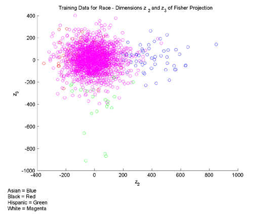
Fig. 3 [larger version]
![[larger version]](images/full/extremaDiff1.png)
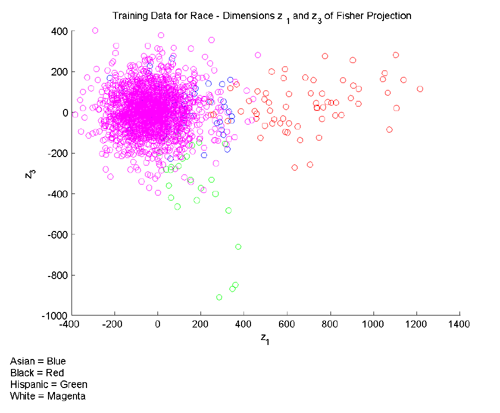
Fig. 3 [larger version]
![[larger version]](images/full/extremaDiff2.png)
Why was it useful?
Multi-GLD was one of the most successful techniques that we attempted. Given suitable support in the form of augmented training data, multi-GLD classification produced very good results on the particularly difficult challenges of race and age classification. See the presentation for extensive documentation of our efforts at applying multi-GLD to race classification.
Neural networks are a particularly trendy classification technique. A neural network is composed of a number of nodes, arranged in layers and connected by links. Each link has a numeric weight associated with it. Weights are the primary means of of long-term storage in the network, and learning takes place by updating the weights [4]. The backpropagation algorithm provides an efficient technique for training the weights in a neural network given a set of labeled examples. Given some modest assumptions, it can be shown that a two-layer neural network is capable of approximating arbitrary decision boundaries.
Figure 5 below presents a schematic representation of a two-layer neural network.
Fig. 5 (Courtesy of [5])
Why did we try NNs?
Neural networks have a certain "black box" appeal. The ready availability of neural net toolboxes combined with the promise of nonlinear decision boundaries makes them a seductive choice for many classification tasks. It was very simple to apply Matlab's neural network functionality to our training data, so we were able to obtain a preliminary set of classification results for most of our features fairly painlessly.
How did we apply NNs?
The neural networks that we used for this project were structured as follows:
- Two layers (not including the input layer).
- Variable number of nodes in the hidden layer. For each feature, we tested networks with between 1 and 20 nodes in the hidden layer.
- Tan-sigmoidal transfer functions in the hidden and output layers.
- One bias node connected to each node in the hidden and output layers.
For training the networks, we used Matlab's implementation of the backpropagation algorithm, which includes support for an adaptive learning rate and momentum in the gradient descent. Networks were trained for 1200 epochs, or until the mean-squared error on the training set fell below a threshold of 0.005.
Was it useful?
The downfall of neural networks is their voracious training requirements. The networks can have a very large number of free parameters, and this number tends to scale poorly with increasing numbers of hidden nodes. Perhaps not surprisingly, we found that neural nets were able to perform well on classes for which there was a large quantity of training data (e.g. white faces or adult faces) but very poorly on classes for which training data was in shorter supply (e.g. black faces or teenage faces). For a more detailed discussion of neural networks as applied to race classification, see the presentation.
Support Vector Machines (SVMs)
Generalized linear discriminant classifier with a maximum-margin fitting criterion. Figure 6 depicts this concept.
Fig. 6 (Courtesy of [3]).
SVMs find the hyperplane h, which separates the training examples from each class with maximum margin. The training points closest to the hyperplane are called Support Vectors (depicted as circles in the figure).
Why did we try SVMs?
Having explored GLD classifiers in detail, we wanted to try SVMs as well for the purposes of comparison. We applied SVMs to a selection of our features (sex, glasses, hat, and bandana) but the computation time required precluded further investigation.
How did we apply SVMs?
Due to time constraints at the end of the project, we did not have an opportunity to investigate SVMs in great detail. In the trials which we did run, we used the OSU SVM toolkit [4] to construct SVMs with a second-degree polynomial kernel.
Was it useful?
In general, SVMs produced results which were no better than the computationally simpler GLD classifiers. Small improvements were obtained on the hat and bandana classifications using SVMs as compared to the original GLD classifications.
As described in the presentation, we experimented with augmenting the original training set with synthetic faces. These synthetic faces were formed from the members of the original training set, and intended to enhance classifier performance by providing additional variation in the training process. Two techniques were used to create synthetic faces.
Mirroring
The rows of pixels in the original faces could simply be flipped in a left-to-right fashion to generate "mirrored" faces. Mirroring represents a conservative approach to generating synthetic faces, and as such has both drawbacks and advantages:
- The advantage of mirroring is that the resulting mirrored face is guaranteed to be a "real" face; that is, the mirroring process will not create artifacts in the resulting synthetic faces that could potentially confuse a classifier.
- The disadvantage of mirroring is that the resulting faces are very similar to their parents. Thus, mirroring alone will increase the variation in the training set only slightly.
Averaging
Sets of faces from a given class could be averaged together to generate new faces for that class. As compared to mirroring, averaging is a more bold technique for generating synthetic faces.
- The advantage of averaging is that it has the potential to generate synthetic faces which are dissimilar to their parents. That is, averaging can increase the variation in the training set much more than a more conservative operation such as mirroring.
- The disadvantage of averaging is that it has the potential to introduce artifacts into the training data which might distract a classifier. For example, if we average just two random faces together, the resulting face will generally look rather frightening, and include large distortions that are not characteristic of real faces.
When employing averaging, we must balance the competing tensions of i) minimizing the appearance of artifacts in the averaged faces, and ii) making the averaged faces reasonably different from one another. The more faces we average together to generate a new face, the smaller the chance of major artifacts, but the more homogeneous the results.
Through a process of empirical experimentation, we determined that averaging the original faces in blocks of six to eight produced synthetic faces with minimal visual distortion and reasonable variation. As a potential avenue for future work, it would be interesting to experiment with techniques for learning the optimal number of faces to average together rather than approximating it via direct observation.
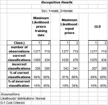
In this section we present a complete tabulation of the classification results which were obtained in the course of this project. The results are divided by feature.
|
Sex was the only class for which we could apply ML. This technique produced almost the same results regardless of whether the priors were derived from the training data or set to be equal. The optimum degree for the polynomial augmentation used with the GLD classifier was determined to be 1; in other words, the GLD classifier is in this case a simple linear discriminant in the original feature space. This observation explains why the results of employing GLD and ML are nearly identical.
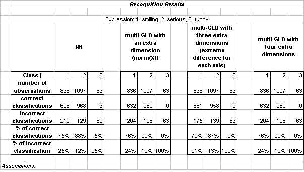 |
Neural Networks (NN) was the only technique which was able to correctly classify any of the faces labeled as "funny". Results are reported for a neural network with 13 hidden nodes. The difficulty of classifying funny faces is not surprising, as the class itself was not terribly well defined. That is, faces were classified as funny if they were neither smiling nor serious; thus, the funny faces did not have strong interclass resemblance.
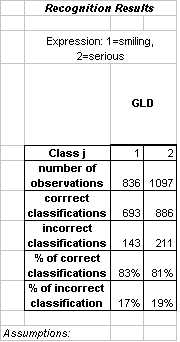 |
The results of two-class expression classification satisfy our optimality criterion well in the sense that both classes, smiling and serious, exhibit high accuracy. Results are reported for a GLD in which the degree of the polynomial augmentation is 2. We were satisfied with these results and decided to move towards more challenging classification problems.
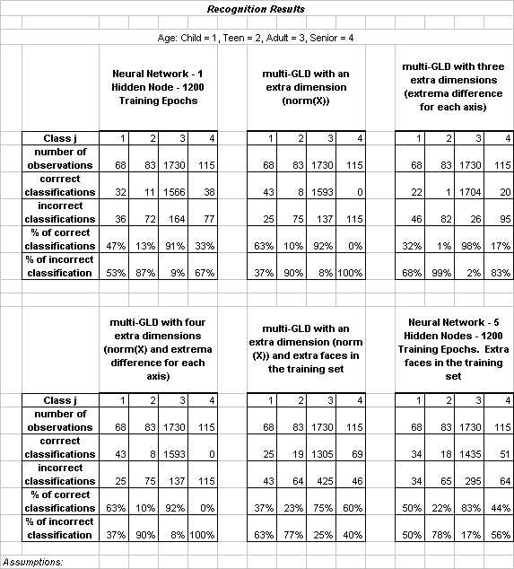 |
Age, like race, was one of our most challenging features. The difficulty was to obtain high accuracy across all of the classes, as opposed to just in the dominant class (adult faces) for which there was a very large quantity of training data. Better results were obtained after augmenting the training data to include synthetic faces, and then applying a neural network to the expanded training set.
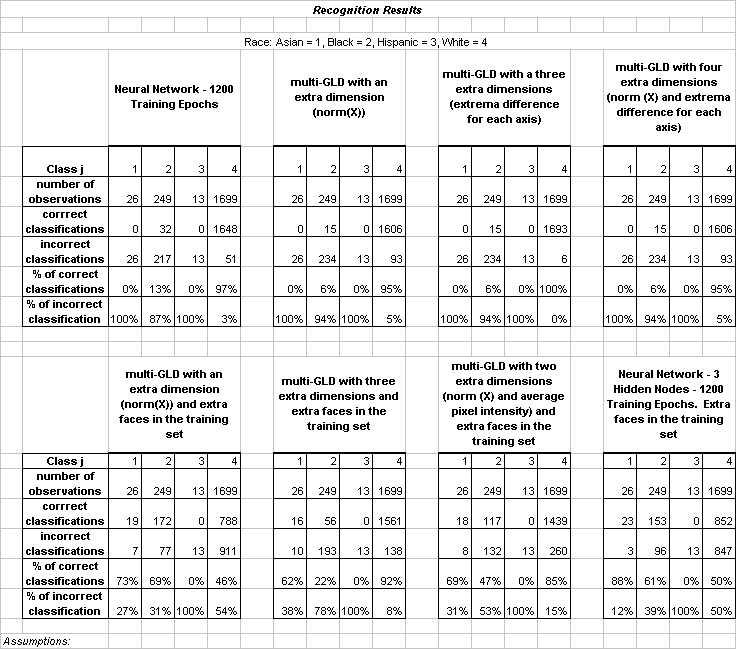 |
A detailed discussion of race is given in the presentation slides.
 |
Results for hat classification by GLD and SVM were very similar. The GLD results are for a classifier with polynomial augmentation of degree 7.
 |
We were not able to obtain good results for bandana using any of the methods we tried. We attribute this fact to the heterogeneity of the class, which includes people wearing bandanas around the head, around the neck and even one person whose "bandana" consisted of a large collar. The GLD results are for a classifier with polynomial augmentation degree of 3.
 |
Again, the use of synthetic faces significantly increased the recognition accuracy for people wearing glasses. It is interesting to note that the synthetic faces generated by averaging other faces in the glasses class tended to have a larger degree of spurious variation than averaged faces in other classes. However, somewhat surprisingly, this variation does not appear to have reduced the usefulness of the synthetic face technique. The GLD classifier used on the original training set had polynomial augmentation degree 7, while the classifier applied to the augmented training set had degree 1.
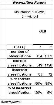 |
Moustache proved to be a relatively simple classification to perform. Results are reported for a GLD classifier with polynomial augmentation degree 4. As with the two-class version of expression, we were satisfied with these initial results and moved on to focus on more challenging features.
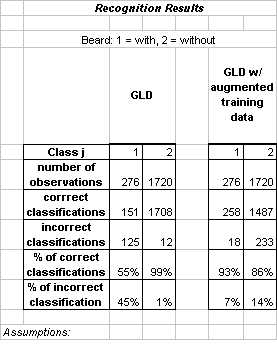 |
The beard class provides the most dramatic example of how synthetic faces can improve recognition accuracy. Both GLD classifiers had a polynomial augmentation degree of 3.
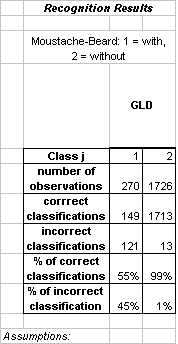 |
There were a considerable number of people with both moustache and beard in the training set. We formed this new class to compare the classification accuracy to the isolated moustache and beard classes. The result obtained using GLD (polynomial augmentation degree 3) is similar to that which was observed for the beard feature. Since augmenting the training data increased the classification accuracy for beard substantially, we think it likely that synthetic faces would also improve classification of the moustache-beard feature.
[1] Belhumeur, P.N., Hespanha, J.P., Kriegman, D.J., "Eigenfaces vs FisherFaces: Recognition Using Class Specific Linear Projection," IEE Trans. Pattern Analysis and Machine Intelligence, 19(7), pp. 711-720, July 1997.
[2] Lawrence, S., Yianilos, P., Cox, I. Face Recognition Using Mixture-Distance and Raw Images, 1997 IEEE International Conference on Systems, Man, and Cybernetics, IEEE Press, Piscataway, NJ, pp. 2016-2021, 1997.
[3] http://www.bus.utexas.edu/faculty/Tom.Sager/BA386T/Post-Mortem(Sep19).doc
[4] http://www.eleceng.ohio-state.edu/~maj/osu_svm/
[5] http://kiew.cs.uni-dortmund.de:8001/mlnet/instances/81d91e8d-dbce3d1e90