The problem & datasets
We are
given a training set of 1997 128 x 128 8-bit gray scale photos of faces, and a
testing set of 1996 similar photos. We are also given two ascii files with
descriptions of these faces in a standard format, which contains (or implies)
entries for nine fields of information, which can take values from a
predetermined discrete set. I will from now on call these fields “labels”,
their index numbers “label indices”, and their content “label values”. These
labels, together with their allowable values are:
LABELS VALUES N
VALUES
labels{1} =
'gender'; values{1,i} = ’male, female’ (2)
labels{2} =
'age'; values{2,i}
= ’child, teen, adult, senior’ (4)
labels{3} =
'race'; values{3,i}
= ’white, black, asian, hispanic, other’ (5)
labels{4} =
'expression'; values{4,i}
= ’serious, smiling, funny’ (3)
labels{5} =
'moustache'; values{5,i}
= ’a, no’ (2)
labels{6} =
'beard'; values{6,i}
= ’a, no’ (2)
labels{7} =
'glasses'; values{7,i}
= ’a, no’ (2)
labels{8} =
'bandana'; values{8,i}
= ’ , no’ (2)
labels{9} =
'hat'; values{9,i}
= ’a, no’ (2)
Thus, all
allowable combinations are in a discrete and finite 9D space.
However,
after converting the ascii file containing the labels to matlab array format,
simple analysis showed (as also expected by commonsense knowledge of the
labels) that the distribution in this space is far from uniform:
Label space dims:2
4 5 3 2 2
2 2 2
Total size:3840
Out of which, nonzero elements:95
I.e. percentage of non-zero:0.02474
I.e.only
2.5% (95 cases) of all possible combinations exist in the training set, and as
expected most combinations that could be excluded by commonsense are indeed not
here (i.e. no women having beards).
Mislabelled data
However,
obviously mislabelled data do exist, for example a woman having a moustache.
Also, many allowable combinations simply happenned not to show up in the set:
for example, there are no hispanic children here, which could well have
existed.
Thus, if
our goal is recognition in the real world, and we know the hard constraints of
the world and are willing to hardcode them, we can either force the system not
to take into account samples with incoherent label values, or treat the labels
based on the prior probabilities of the possible solutions of their
inconsistency (assuming single error etc.).
Else, we
can let the system learn the allowable combinations based on what has seen:
thus, it might mistakingly attach a small prior to women with moustaches, which
will eventually flatten out with a large enough training set. And, before
having seen a hispanic child, it might assume that no such a thing does not
exist. Here, fortunately we can easily incorporate the fact that such a
combination might arise in subsequent training data in a non-crisp
probabilistic framework (for the case of online training or cumulatively
trainable systems).
Unfortunately,
subjectivity and operator errors enter the picture in labelling, too, and this
is apparent if we consider for example the distinction between serious and
smiling in this set, and futhermore (this was really problematic) what a beard
really is!…
A fundamental choice: categories,
partitioning & their distribution among classifiers
Here, a
fundamental decision must take place. After excluding (or not) obviously
incoherent combinations, how do we arrange the remaining allowable cases?
Should we preserve the original 9D setting? Or should we just flatten them out
in 1D? Or maybe repartition them in a different way? Is there anything to gain
from this?
Let’s
examine how classifiers enter the picture. Discriminative classifiers will
dichotomise (or partition, in the multicategory case) the set of allowable
outputs into subsets and will decide which subset is more probable (in the
crisp version). In a less crisp case, they will attach a confidence value to
each subset. Generative models will
give a confidence value that the input sample came from a specific subset of
the allowable cases. If we have a dense enough arrangement of classifiers
and/or models, in a suitable topology, we can get increasingly fine-grained in
our decision and null down to the most probable single-element subset, leading
us to a full answer. In general, we should evaluate all possible evidence given
by our classifiers and the priors, and reach a decision, probably with an
approach similar to a Bayes net. Their might even be cases when we are still
coarse grained or inconfident, so we might be able to resample the world to get
closer to a decision (i.e. ask a clarification question in dialogue, have a
second or better look at a face in face recognition). Of course, here there’s
only one training set, and that’s all.
The moral
of the above is obvious: there are many possible repartitions, and arrangements
of classifiers over these, and even cases of combining classifier outputs
toward the final question. Also, “merging” and “splitting” of classifiers
naturally enters the picture from the design point of view. So how can we be
more specific?
Here, as
this would be out of the scope of the project, we are not attempting to model
the full problem, although it is highly interesting and relevant, and is
definetely worth further theoretical and experimental investigation. So, we’ll
just start with very simple things.
The full and marginalised
priors
In our
case, we have a simple arrangement of nine independent modules, operating
across each of the nine natural dimensions, and thus getting down to
single-element subset granularity. This topology might be at a disadvantage if
the output of each module is crisp: we will be able to incorporate
“marginalised” priors for the values of each dimension, but not the full priors
of the 9D combinations! If the outputs of each module are probabilities, we can
do a bit better, and reach the decision at a final stage after taking into
account more information. This is a natural next step to possible extensions of
this project.
Of course,
all this depends on what our objective: if we want to maximise recognition rate
as a whole, or the recognition rate of each individual module (where the full
priors don’t enter the picture). Or we might even be counting single errors,
double errors, wanting to consider loss functions etc. Here, we’ll again choose the simplest to
start with: minimum error rate for each individual dimension. But let’s have a
look at the priors:
Below are
the top ten cases of the training set, together with their priors:
1_15%_female-adult-white-smiling-no moustache-no
beard-no glasses-no bandana-no hat-
2_12%_male-adult-white-serious-no moustache-no
beard-no glasses-no bandana-no hat-
3_11%_male-adult-white-smiling-no moustache-no
beard-no glasses-no bandana-no hat-
4_10%_female-adult-white-serious-no moustache-no
beard-no glasses-no bandana-no hat-
5_7%_male-adult-white-serious-with moustache-no
beard-no glasses-no bandana-no hat-
6_4%_male-adult-white-smiling-with moustache-no
beard-no glasses-no bandana-no hat-
7_4%_female-teen-white-smiling-no moustache-no
beard-no glasses-no bandana-no hat-
8_4%_male-child-white-serious-no moustache-no beard-no
glasses-no bandana-no hat-
9_4%_male-child-white-smiling-no moustache-no beard-no
glasses-no bandana-no hat-
10_3%_male-teen-white-smiling-no moustache-no beard-no
glasses-no bandana-no hat-
The top 10 cases cover:74
Notice that
we have covered almost 75% with the top 10, and the rest is covered by the
remaining 85 cases. Also, notice how commonsense stereotypes have arisen:
smiling white female adults, and serious white male adults dominate… J
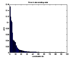
Below are
the full priors in descending order:

Figure 1: the full priors of the training set
(roughly similar in test)
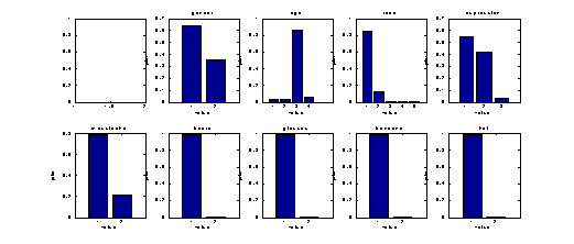
The
marginalised priors follow:

Figure 2: the marginalised priors of the
training set

Figure 3: the marginalised priors of the
testing set.
Some
obvious points to notice:
- Every label except gender and
expression has very imbalanced priors, much more for the last four. (high
entropy).
- There is considerable difference of
the marginalised priors between the train and test sets, and so they are
somewhat mismatched for recognition, even at a very fundamental level. Taking
into account the size of the samples (2K), this difference seems significant
statistically. Other evidence might also signal this; for example, mean face
and eigenvector differences, or mutual recognition rates etc.
- By the trivial classification rule
of just choosing the value having the largest prior of the training set, we can
get on the test set:
0.6398 0.8667
0.8512 0.5496 0.7876
0.9950 0.9960 0.9960
0.9900
which definetely are high
percentages, and thus any results should be considered ABOVE this baseline…
Pairs of labels
By
considering only pairs of labels, and their marginalised priors, we can gain
some insight in combining outputs of pairs of classifiers (instead of going to
the full 9D problems). For example, just by detecting zeros in the 2D priors,
we can get automatised statements of the form:
Facts I know about the relation of_gender_with_beard:
-> Noone_with_female_gender_also_has_a_beard!-
And these
might be worth exploiting, if for example we have a highly robust moustache
classifier correcting a mediocre gender decision and vice versa, or even in
more balanced cases given not highly overlapping errors. This argument can go a
bit further (considering pairs again), and the mutual information of their
priors shows such “inbalanced” cases that can easily be exploited (again
depending on their individual classifier performance and matching). For pairs,
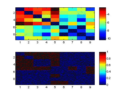
we get:

Figure 4: mutual information of priors
(upper figure: color coded log of mutual, for
pairs of labels,
lower figure: thresholding of the above)
It is thus
apparent which pairs of features offer useful information about each other:
(1,5)=(gender,
moustache) has the highest score, but also (expression, gender) etc.
Thus, if we
don’t wanna consider the full priors, and maybe just have crisp-output independent
classifiers, we can still exploit this information, as we will do later, albeit
in a very superficial way.