Images, preprocessing
& representations
The images
Unfortunately
the images are of bad quality, but in the real world this might be all that is
available. Some of them have a periodic vertical translation; some of them have
very bad picture quality, others have strange and extreme rotations, often hair
and backgorund unite, and there is large absolute intensity and contrast
variation. Others are even totally uniform (2104, 2105, 2106). Some typical
examples follow:
|
|
|
|
|
|

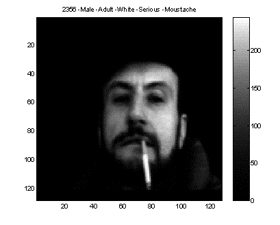
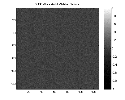

Figure 5: Examples of bad and mislabelled
images
Thus, one
might want to consider detecting and omitting outliers. One simple method would
be to consider manually going through the images that have the greatest
distance from either the center of the set, or centers of category clusters in
principal components space.
Here, we
haven’t omitted outliers in order to provide performance results comparable to
others.
Preprocessing
Apart from
possible corrections in mismatched labels and omission of faulty outliers, some
forms of image preprocessing might prove crucial in increasing recognition
performance. These might be: image rectangle alignment (fortunately, faces are
not really misaligned in our datasets), rotation compensation, illumination
compensation, contrast adjustments etc. These were unfortunately not tried out
here, as they form considerable problems their own right, even more so when the
input is only 2D grayscale pictures.
However,
one simple form of preprocessing that we used was zeroing all pixels with
intensities below a threshold in the mean face image. Thus, we effectively had
an almost elliptical mask, extending also towards the neck. This is generally
an advantage, although the some of the cut out region might have proved useful
for example for hat detection.
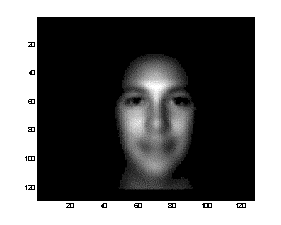
Figure 6: The face mask used
Representations
Choice of
representation is another important matter. Here we have as compact as possible
a representation, summarising the information relevant for good separation. Feature
selection will then follow, and select and even smaller subset. Some obvious
choices that were tried out were:
- Multiresolution images: 128 x 128
(original), 64 x 64, 32 x 32 down to 16 x 16. Interpolation is a question here;
however, its choice doesn’t seem to have a significant effect – simple 2x2
averaging will do.
- PCA of the above: some of the
numerical problems in higher resolutions, were eliminated in the lower ones.
Qualitative correspondance of eigenvectors of course exists, and we get similar
projections
- Cut regions of the above resized
images, and their pca’s: for example, a region around the mouth for moustache
and expression, and a region around the eyes for glasses.
- DCT’s of sliding overlapping
windows, possibly with filtered out DC and high frequencies: only briefly used
in embedded HMM’s (details follow later). DCT approximates PCA, fast algorithms
exist, and as is independent of the training set.
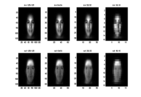
Figure 7: Mean Face and first eigenvect
(hair-related) at various resolutions