Classification of Sleep Data
<Akane Sano>
Objectives
Generally, sleep
pattern is evaluated with polysomnography in a sleep lab.
EEG is mainly used to
evaluate sleep stages and many studies have been done to estimate
sleep stages automatically with
EEG, motion, heart rates.
Recent studies have
shown that sleep patterns depend on not only sleep quality, but also other
factors such as
memory consolidation, sleep loss
and immune system. On the other hand, researchers have investigated on
electrodermal activity (EDA)
during sleep. EDA is a skin conductance that is related to sympathetic
activity.
This project aims to quantify
electrodermal activity during sleep and evaluate the relationship between sleep
stage and EDA.
Methods
(1)
Data
Data
we used for this project were recorded with healthy students and the detail is
as follows.
•
Healthy
students (N=7)
•
Electroencephalogram(EEG)
100Hz
•
Electro
dermal activity(EDA) 32Hz
•
Motion 32Hz
•
Labels
: sleep stages (every 30s)
(Wake, REM, NonREM1-4,
Movements/Noise)
In order to simplify the problem,
we combined labels of NonREM1-4 into on stage, NREM and got four classes:
Wake, REM, Non-REM,
Movements/Noise.
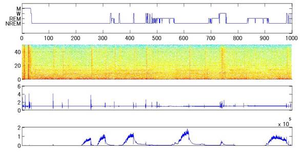
Figure 1 Time
series data during sleep
(1)
Pre-processing
Electrodermal
activity was low-pass filtered and motion data was band-pass filtered.
(2)
Feature
Extractions
All signals were segmented
into 30s window and features shown below were all computed with MATLAB.
•
EEG
:
–
Frequency
Energy
•
delta:0.5-4,Hz
•
theta:4-8
•
alpha:8-13Hz
•
beta:13-40Hz
•
gamma:40-50Hz)
•
Motion:
–
Average
of Amplitude
–
Standard
Deviation of Amplitude
–
Zero-crossing
•
EDA
:
–
Average
of Amplitude (Normalized)
–
Standard
Deviation of Amplitude
–
#
of peaks
–
Gradient
–
Frequency
Energy(0-0.5Hz, every 0.1Hz)
•
Elapsed
Time (0:Start-1:End of Data)
Table 1 The number of samples for each class
|
Subject |
WAKE |
REM |
NREM |
MOVEMENT |
|
Q |
317 |
124 |
527 |
0 |
|
R |
15 |
141 |
719 |
3 |
|
S |
46 |
184 |
714 |
9 |
|
T |
10 |
189 |
630 |
0 |
|
U |
51 |
209 |
709 |
3 |
|
V |
38 |
203 |
703 |
5 |
|
W |
49 |
179 |
735 |
32 |
|
% |
8.0 |
18.8 |
72.4 |
0.8 |
Figure
2 Electrodermal activity during sleep
Figure 3 Example of
features (Red Non-REM, blue Wake, pink REM black M)
(3)
Machine
Learning
Using Matlab,
different machine learning methods were compared.
A)
K-Nearest
Neighbors (k=1-200)
B)
Support
Vector Machine (libSVM)
1.
Kernel
I.
Linear
II.
Polynomial
III.
Radial
Basis Function
2.
Feature
I.
Static
Feature (30s window)
II.
Dynamic
features (150s, 300s, 450s, 600s window)
C)
Neural
Network (One lawyer, n=2-20)
(4)
Evaluation
Leave one subject out was
performed and F-measures for each class were compared in classification methods
and features.
Although
accuracy was compared in the final presentation, f-measure was computed in order
to consider
all
aspectis of true positive, false positive, true negative and false negative.
Because time was ran out,
f-measure for k Nearest Neighbors could not be illustrated here.
Results
First, features except
elapsed time were used for classification.
F-measures were compared for
features in 4 classes.
A)
SVM
Table
2 F measures with different
features and kernels
|
Class |
|||||
|
Kernel |
Feature |
W |
R |
NR |
M |
|
Linear |
EEG |
0.31 |
0.23 |
0.82 |
0.00 |
|
ALL |
0.28 |
0.35 |
0.83 |
0.00 |
|
|
EDA |
0.00 |
0.00 |
0.84 |
0.00 |
|
|
MOTION |
0.00 |
0.00 |
0.84 |
0.00 |
|
|
Poly |
EEG |
0.00 |
0.00 |
0.84 |
0.00 |
|
ALL |
0.01 |
0.00 |
0.84 |
0.00 |
|
|
EDA |
0.00 |
0.00 |
0.84 |
0.00 |
|
|
MOTION |
0.00 |
0.00 |
0.84 |
0.00 |
|
|
RBF |
EEG |
0.22 |
0.07 |
0.81 |
0.00 |
|
ALL |
0.12 |
0.05 |
0.83 |
0.00 |
|
|
EDA |
0.00 |
0.00 |
0.84 |
0.00 |
|
|
MOTION |
0.00 |
0.00 |
0.84 |
0.00 |
|
As can been seen in Table
2, the polynomial kernels the largest F-measures for N-REM,
But Linear Kernel represented the
largest averaged F-measures.
In addition, All 4 features
showed more than 0.8 of F-measures in NREM, but
only EEG and ALL features could
classify Wake and REM with 0.2-0.3 of F-measures.
EDA and Motion did not work in
classification of Wake, REM and Motion.
Table
3 F measures with different features and kernels (Elapsed Time Added)
|
With
Elapsed Time |
Class |
||||
|
Kernel |
Feature |
W |
R |
NR |
M |
|
Linear |
EEG |
0.26 |
0.28 |
0.83 |
0.00 |
|
ALL |
0.21 |
0.38 |
0.83 |
0.00 |
|
|
EDA |
0.00 |
0.00 |
0.84 |
0.00 |
|
|
MOTION |
0.00 |
0.00 |
0.84 |
0.00 |
|
|
Poly |
EEG |
0.00 |
0.00 |
0.84 |
0.00 |
|
ALL |
0.02 |
0.00 |
0.84 |
0.00 |
|
|
EDA |
0.03 |
0.00 |
0.83 |
0.00 |
|
|
MOTION |
0.00 |
0.00 |
0.84 |
0.00 |
|
|
RBF |
EEG |
0.23 |
0.12 |
0.82 |
0.00 |
|
ALL |
0.16 |
0.05 |
0.83 |
0.00 |
|
|
EDA |
0.01 |
0.00 |
0.83 |
0.00 |
|
|
MOTION |
0.00 |
0.00 |
0.84 |
0.00 |
|
Table 3 showed F
measures with different features and kernels after Elapsed Time was added.
As shown in Table 3, the feature
of elapsed time improved F-measures in most cases.
Next, for linear
kernel, we applied dynamic features with different length of window.
In table 2 and 3, we used static
features from 30s windows, however we assumed that
temporal information sleep would
improve classification because the sleep pattern has
a temporal structure, for example 90
minutes cycle of REM and NREM.
We used time-series features for
classification.
Tables 4 showed the
comparison of F measures in different features and window length
of dynamic features. The dynamic
features improved F-measures except N-REM classes
compared to the results with
static features in table 1.In comparison of window length,
each class and feature had
different optimal length of windows.
Table 4: F measures with different
features (with Linear Kernel and Dynamic features)
|
Class |
|||||
|
Window
Length |
W |
R |
NR |
M |
|
|
EEG |
150s |
0.38 |
0.48 |
0.82 |
0.00 |
|
300s |
0.38 |
0.49 |
0.82 |
0.00 |
|
|
450s |
0.36 |
0.50 |
0.82 |
0.00 |
|
|
600s |
0.32 |
0.51 |
0.82 |
0.00 |
|
|
ALL |
150s |
0.37 |
0.49 |
0.82 |
0.00 |
|
300s |
0.36 |
0.47 |
0.82 |
0.00 |
|
|
450s |
0.34 |
0.47 |
0.82 |
0.00 |
|
|
600s |
0.30 |
0.46 |
0.82 |
0.00 |
|
|
EDA |
150s |
0.00 |
0.00 |
0.84 |
0.00 |
|
300s |
0.00 |
0.00 |
0.84 |
0.00 |
|
|
450s |
0.00 |
0.00 |
0.84 |
0.00 |
|
|
600s |
0.00 |
0.00 |
0.84 |
0.00 |
|
|
MOTION |
150s |
0.01 |
0.00 |
0.84 |
0.00 |
|
300s |
0.06 |
0.00 |
0.84 |
0.00 |
|
|
450s |
0.06 |
0.00 |
0.84 |
0.00 |
|
|
600s |
0.06 |
0.00 |
0.84 |
0.00 |
|
D)
Neural Network
As shown in table 5,
most cases improved and F-measures as the number of nodes increase;
however, in EEG features
F-measures decreased.
F-measures saturated as the
number of nodes increases.
Table 5: F measures with
different # of nodes and features
|
EEG |
ALL |
|||||||
|
# |
W |
R |
NR |
M |
W |
R |
NR |
M |
|
2 |
0.71 |
0.72 |
0.91 |
0.12 |
0.62 |
0.67 |
0.91 |
0.17 |
|
4 |
0.70 |
0.72 |
0.90 |
0.11 |
0.70 |
0.69 |
0.91 |
0.16 |
|
6 |
0.70 |
0.72 |
0.90 |
0.11 |
0.71 |
0.70 |
0.91 |
0.16 |
|
8 |
0.69 |
0.72 |
0.90 |
0.13 |
0.72 |
0.70 |
0.91 |
0.15 |
|
10 |
0.69 |
0.72 |
0.90 |
0.12 |
0.72 |
0.71 |
0.91 |
0.16 |
|
12 |
0.69 |
0.72 |
0.90 |
0.11 |
0.72 |
0.71 |
0.91 |
0.19 |
|
14 |
0.69 |
0.72 |
0.90 |
0.13 |
0.72 |
0.71 |
0.91 |
0.20 |
|
16 |
0.69 |
0.72 |
0.90 |
0.13 |
0.72 |
0.72 |
0.91 |
0.21 |
|
18 |
0.68 |
0.72 |
0.90 |
0.13 |
0.72 |
0.72 |
0.91 |
0.20 |
|
20 |
0.68 |
0.72 |
0.90 |
0.14 |
0.72 |
0.72 |
0.92 |
0.21 |
|
EDA |
MOTION |
|||||||
|
# |
W |
R |
NR |
M |
W |
R |
NR |
M |
|
2 |
0.21 |
0.00 |
0.80 |
0.00 |
0.31 |
0.00 |
0.81 |
0.01 |
|
4 |
0.21 |
0.00 |
0.80 |
0.00 |
0.32 |
0.00 |
0.81 |
0.01 |
|
6 |
0.24 |
0.00 |
0.81 |
0.00 |
0.32 |
0.00 |
0.81 |
0.01 |
|
8 |
0.25 |
0.00 |
0.81 |
0.00 |
0.32 |
0.00 |
0.81 |
0.01 |
|
10 |
0.25 |
0.00 |
0.81 |
0.00 |
0.32 |
0.00 |
0.82 |
0.01 |
|
12 |
0.24 |
0.00 |
0.81 |
0.00 |
0.32 |
0.00 |
0.82 |
0.01 |
|
14 |
0.24 |
0.00 |
0.82 |
0.00 |
0.32 |
0.00 |
0.82 |
0.01 |
|
16 |
0.24 |
0.00 |
0.82 |
0.00 |
0.32 |
0.00 |
0.82 |
0.01 |
|
18 |
0.24 |
0.00 |
0.82 |
0.00 |
0.32 |
0.00 |
0.82 |
0.01 |
|
20 |
0.24 |
0.00 |
0.82 |
0.00 |
0.32 |
0.00 |
0.82 |
0.01 |
In
table6, we compared F-measures in different features.
Feature ALL showed the largest
F-measure.
EDA and MOTION could classify
samples in wake and REM classes, while
they did not work in SVM.
Table 6: F measures with
different # of nodes and features (n=20)
|
Class |
|||||
|
W |
R |
NR |
M |
||
|
Features |
EEG |
0.70 |
0.74 |
0.91 |
0.00 |
|
ALL |
0.79 |
0.75 |
0.92 |
0.40 |
|
|
EDA |
0.48 |
0.00 |
0.83 |
0.00 |
|
|
MOTION |
0.31 |
0.00 |
0.82 |
0.06 |
|
As
can been seen in table 7, F-measures improved by adding the feature of elapsed
time,
especially in MOVEMENT class, on
the other hand, F-measures in Movement decreased.
Table 7: F measures with
different # of nodes and features (n=20) (Elapsed Time Added)
|
Class |
|||||
|
W |
R |
NR |
M |
||
|
Features |
EEG |
0.76 |
0.76 |
0.92 |
0.22 |
|
ALL |
0.79 |
0.77 |
0.93 |
0.23 |
|
|
EDA |
0.56 |
0.00 |
0.84 |
0.00 |
|
|
MOTION |
0.47 |
0.05 |
0.82 |
0.26 |
|
Discussions
In SVM, linear kernel
showed the largest F-measure.
We assumed that non linear
kernels than linear kernel showed the better results,
but this might be due to the fact
that the default parameters for polynomial and RBF we used here
was not optimal. We should
compare different parameters in polynomial and RBF.
In addition, wake,
REM, Movement were misclassified into N-REM.
Unequal sample number and overlap
in feature vectors seem to account for this.
Although different weights for
classes were tested in SVM, it did not improve the results.
For this project, classes were
simplified into 4 (Wake, REM, NonREM, Movement), however
NonREM 1-4 had different
characteristics especially in frequency bands and they should be
split into shallow (NonREM 1-2)
and deep sleep (NonREM 3-4) in the future work.
EDA
and motion did show lower F-measures than EEG. Although neural network improved
the F-measures in EDA and motion
shown in table 7, EDA could not show improvement
in REM and MOVEMENT at all.
Several factors can be considered. First, samples of movement
was much smaller than others.
Moreover, EDA during NonREM and wake tends to be large and
have peaks, however sometimes
they had similar characteristics to EDA in REM and MOVEMENT,
where amplitude is small and no
peaks happen. In addition, EDA sometimes started increasing and
decreasing during REM. It might
be hard to discriminate features used for this project. Therefore,
different features such as
duration of peaks and the elapsed time after the previous storm and temporal
model might be useful to classify
REM properly. Furthermore, several studies indicated EDA is more
likely to appear during deep
sleep stages, however some studies have shown that EDA did distinguish
wake and sleep and determine the
sleep onset, but it could not be used to identify sleep stages.
Neural
network showed the largest F-measure compared to other classifiers.
This is because feature vectors
were complex and overlapped. Optimal parameters for wake and REM classes
might be required to improve the
F-measure in non-linear kernels of SVM.
Elapsed
time and dynamic features improved some F-measure. This may be due to the fact
that
sleep pattern is likely to show
temporal structure. However, these temporal features should be optimized or
different temporal structure
might show better generalization. In dynamic features, the longest window
might lead the over-fitting.
Moreover, the feature of elapsed time might not be able to consider the
individual
difference of sleep patterns.
Conclusions
EDA and Motion showed less
accuracy to estimate the sleep stage than EEG and ALL and Wake.
In
comparison of machine learning methods, neural network showed the best accuracy
Elapsed
Time and dynamic features might be effective
Future Work
As sleep patterns
contain the temporal structure, temporal models such as hidden marcov model
and dynamic baysian network might
show better results. In addition, parameters for SVM should be optimized.