Automatic Drum Samples Classification

A final project for Pattern Recogintion MAS 622J/1.126J

Eyal Shahar, MIT Media Lab

All quotes are taken from the the sketch "More Cowbell" as performed in "Saturday Night Live"

Background

Musicians today, both professional and hobbyist, who rely heavily on their computers to make music, usually find themselves with hard drives full of music samples of all sorts. The majority of these samples are of individual drum samples, often called “hits” or “one shots”. Arranging these samples in folders is usually done manually by listening to every sample and moving it into a desired folder. While in the process of making music, retrieval of these samples is done, once more, by tedious auditions of each and every sample. This project is a first step towards making the life of the computer-based musician a little bit easier by automatically classifying these samples and allowing better methods of retrieval.

Objective

The goal of this project is to automatically classify drum samples, compare classification techniques and optimal features sets.

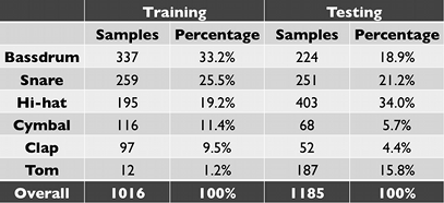
Training And Testing Sets

The training set consists of 1000 samples, divided to 6 classes: bassdrums, snares, hi-hats, cymbals, tom-toms and claps.
The testing set consists of 1200 samples.
The following table describes the distribution of the sets.

Features

Most of the feature extraction was done using the MIRtoolbox for Matlab, by the University of Jyväskylä. These are:

• Brightness – Percentage of energy above 1500Hz
• Rolloff – Frequency below which 85% of the energy is found
• Roughness – based on the frequency ratio of each pair of sinusoids
• Irregularity – degree of variation of successive spectrum peaks
• MFCC – Mel frequency cepstrum coefficients

In addition, two more features were extracted using custom algorithms:

• Pitch – The samples are sliced into equal length frames. In each frame the peak of the spectrum is found. These are averaged and the frequency correlating to that FFT bin is returned.
• Decay – The amplitude envelope of the sample is calculated with MIRtoolbox. The peak amplitude is found, and the decay time is calculated as the time that the amplitude drops from the peak to 50%.

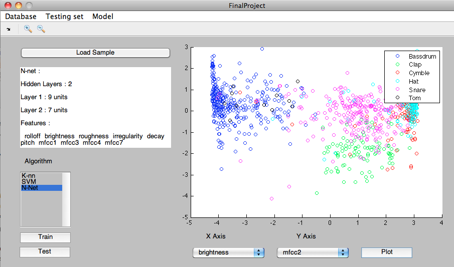
The Matlab GUI

To manage the learning and testing processes, a Matlab GUI was created. It provides quick and intuitive access to feature extraction, loading and saving of the training and testing data sets, saving and loading of classification models, selection of active model, calling the testing and learning routines and graphic visualization of the feature space.

Classification methods

Support vector machine

For this method Matlab’s SVM tools were used. The main drawback of this implementation is that with the absence of the optimization package, as in my computer, the algorithm uses a linear kernel.

Six SVM were trained, one for each class, using a one-versus-all approach.

For validation a leave-one-out method was used.

K Nearest Neighbors

custom KNN algorithm was written for this method and was trained to find the optimal K for 1<k<15 for odd values of k. Validation was done using a leave-one-out approach.

Neural Network

Matlab’s neural networks tools were used for this algorithm, testing both one and two hidden layers, with each layers tested for 5 to 10 units. Validation is a part of the toolbox’s features and therefore no additional validation was done, while the MSE as calculated during the learning process was used as a measure of performance to determine the best net and features set configuration.

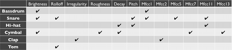
Feature Selection

In all the classification methods learning process, forward feature selection was implemented: At first, the algorithm was with one feature as input. The feature that performed best remained in the features set the algorithm was tested again with each of the remaining features as a second feature. This process repeated it self until the performance did not show improvement of over 0.5%.

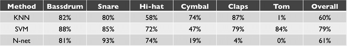
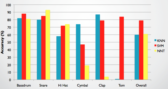
Results And Performance

The K-nearest neighbors gave the best results with k = 9. The selected features were Brightness, Irregularity, Decay, MFCC 1, MFCC 2, MFCC 3 and MFCC 5.

The neural-network learning algorithm produced a 2 hidden layer network, with 9 and 7 units respectively.

The SVM learning algorithm found these features to be optimal:

The following table and graph show the accuracy of detection of the testing set:

Conclusions

Random Insights

• It is interesting to see how features are selected for each of the SVM instances, and to note that theses features do indeed say a lot about the behavior of samples from each class. Hi-hats, for examples, are very short and high pitched, and indeed "Decay" and "Pitch" are among the selected features. Cymbal sounds, on the other hand, are usually very long, noisy and have plenty of high frequencies, so we see "Decay", "Roughness" and "Brightness" selected.
• It is clear that classes that were less common in the training set, namely Toms and Claps, were detected less accurately during testing. The extreme case is of the Toms, of which there were only 12 in the training set, and had negligible detection rates in both k-NN and neural-network algorithms. Furthermore, the performance of the neural network for each class seems to depend heavily on the amount of samples from that class present in the training set. It is therefore important to have enough samples of each class, preferably with all classes equally represented.
• The apparent reason for the SVM algorithm to be an exception is that it has the advantage of producing a different decision machine for each class, and thus has the opportunity to isolate the class unique characteristics, even when a small training set is introduced.

Possible Improvements

The following steps can be considered in order to improve recognition results :

• Extend and manually validate training set - It is very likely that significantly better results can be achieved by enlarging the training set. Also, some samples have been noticed to have dubious character. These, perhaps, should not be a part of the training set.
• Try temporal features approaches, namely HMM - Certain features, such as pitch and MFCC, can give better results when calculated for small time frames. Moreover, their behavior over time can give more information about the sound's class.
• Implement multiple algorithms and majority selection - It is clear that some algorithms are better at detecting certain classes than others. In fact, for every class there is an algorithm the performs very well. Applying all algorithms and taking a joint decision might exhibit better performance.

Future Work

As stated earlier, this work can be a framework of a system with stronger capabilities, such as:

• Melodic instruments samples - Should these algorithms mature into being reliable at a high degree, it would be interesting to see whether they can be applied to melodic instruments.
• Naive retrieval methods - having a database of sounds and their features provides the user with new ways to retrieve sounds. The user would be able to select a sound, and "stroll around" that sound's environment, knowing that these sounds are close to the one he selected.
• Subjective features extraction - Having the user define new features and figuring out how these features are reflected in the existing features can give fascinating results. Suppose a user teaches the machine what sounds are "duller" than others, "sharper", more "soothing", or "yellow". Then musicians can retrieve sounds from the based on their subjective definitions.